Wyszukaj w skryptach "stoch"

Stochastic Momentum+HistogramI modified SMI from UCSGear by adding histogram into his code. I personally use it as a slow SMI, 5,10 to find divergences and gauge the trend's stregth. This indicator is pretty useful for finding entry and exit when the price hit support or resistance in low timeframe.
I find histogram divergence to be useful as you can really see into more detail when the trend strength is waning.
I hope you like it :)


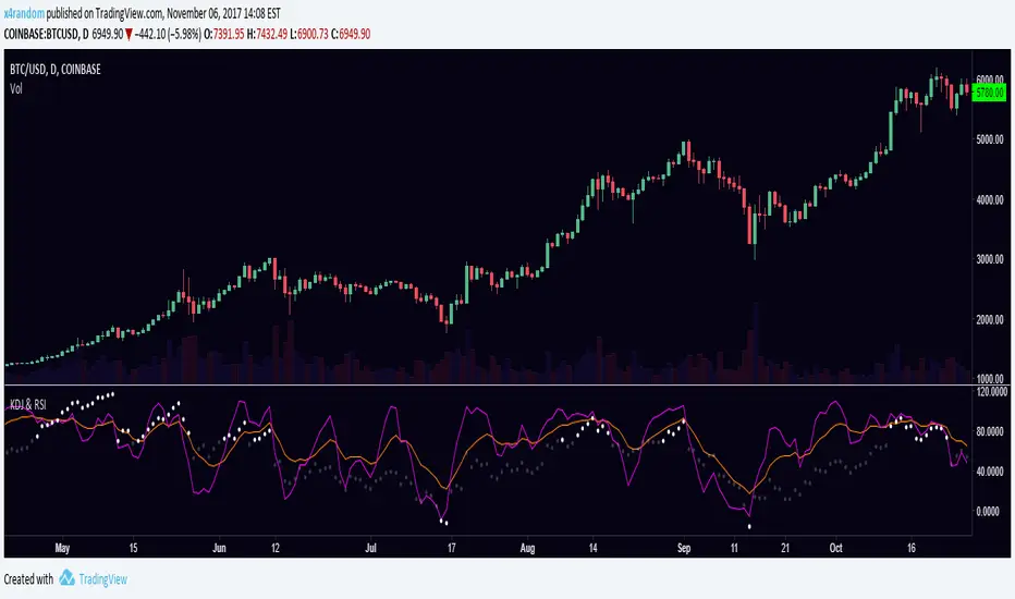
KDJ & RSIRSI and KDJ indicator combined.
KDJ: Buy when J (purple) is going up and and crossing KD (orange) from below. Sell vise versa.
RSI: Overbought when RSI is over 70, oversold when RSI is under -10.


Market Spiralyst [Hapharmonic]Hello, traders and creators! 👋
Market Spiralyst: Let's change the way we look at analysis, shall we? I've got to admit, I scratched my head on this for weeks, Haha :). What you're seeing is an exploration of what's possible when code meets art on financial charts. I wanted to try blending art with trading, to do something new and break away from the same old boring perspectives. The goal was to create a visual experience that's not just analytical, but also relaxing and aesthetically pleasing.
This work is intended as a guide and a design example for all developers, born from the spirit of learning and a deep love for understanding the Pine Script™ language. I hope it inspires you as much as it challenged me!
🧐 Core Concept: How It Works
Spiralyst is built on two distinct but interconnected engines:
The Generative Art Engine: At its core, this indicator uses a wide range of mathematical formulas—from simple polygons to exotic curves like Torus Knots and Spirographs—to draw beautiful, intricate shapes directly onto your chart. This provides a unique and dynamic visual backdrop for your analysis.
The Market Pulse Engine: This is where analysis meets art. The engine takes real-time data from standard technical indicators (RSI and MACD in this version) and translates their states into a simple, powerful "Pulse Score." This score directly influences the appearance of the "Scatter Points" orbiting the main shape, turning the entire artwork into a living, breathing representation of market momentum.
🎨 Unleash Your Creativity! This Is Your Playground
We've included 25 preset shapes for you... but that's just the starting point !
The real magic happens when you start tweaking the settings yourself. A tiny adjustment can make a familiar shape come alive and transform in ways you never expected.
I'm genuinely excited to see what your imagination can conjure up! If you create a shape you're particularly proud of or one that looks completely unique, I would love to see it. Please feel free to share a screenshot in the comments below. I can't wait to see what you discover! :)
Here's the default shape to get you started:
The Dynamic Scatter Points: Reading the Pulse
This is where the magic happens! The small points scattered around the main shape are not just decorative; they are the visual representation of the Market Pulse Score.
The points have two forms:
A small asterisk (`*`): Represents a low or neutral market pulse.
A larger, more prominent circle (`o`): Represents a high, strong market pulse.
Here’s how to read them:
The indicator calculates the Pulse Strength as a percentage (from 0% to 100%) based on the total score from the active indicators (RSI and MACD). This percentage determines the ratio of circles to asterisks.
High Pulse Strength (e.g., 80-100%): Most of the scatter points will transform into large circles (`o`). This indicates that the underlying momentum is strong and It could be an uptrend. It's a visual cue that the market is gaining strength and might be worth paying closer attention to.
Low Pulse Strength (e.g., 0-20%): Most or all of the scatter points will remain as small asterisks (`*`). This suggests weak, neutral, or bearish momentum.
The key takeaway: The more circles you see, the stronger the bullish momentum is according to the active indicators. Watch the artwork "breathe" as the circles appear and disappear with the market's rhythm!
And don't worry about the shape you choose; the scatter points will intelligently adapt and always follow the outer boundary of whatever beautiful form you've selected.
How to Use
Getting started with Spiralyst is simple:
Choose Your Canvas: Start by going into the settings and picking a `Shape` and `Palette` from the "Shape Selection & Palette" group that you find visually appealing. This is your canvas.
Tune Your Engine: Go to the "Market Pulse Engine" settings. Here, you can enable or disable the RSI and MACD scoring engines. Want to see the pulse based only on RSI? Just uncheck the MACD box. You can also fine-tune the parameters for each indicator to match your trading style.
Read the Vibe: Observe the scatter points. Are they mostly small asterisks or are they transforming into large, vibrant circles? Use this visual feedback as a high-level gauge of market momentum.
Check the Dashboard: For a precise breakdown, look at the "Market Pulse Analysis" table on the top-right. It gives you the exact values, scores, and total strength percentage.
Explore & Experiment: Play with the different shapes and color palettes! The core analysis remains the same, but the visual experience can be completely different.
⚙️ Settings & Customization
Spiralyst is designed to be highly customizable.
Shape Selection & Palette: This is your main control panel. Choose from over 25 unique shapes, select a color palette, and adjust the line extension style ( `extend` ) or horizontal position ( `offsetXInput` ).
scatterLabelsInput: This setting controls the total number of points (both asterisks and circles) that orbit the main shape. Think of it as adjusting the density or visual granularity of the market pulse feedback.
The Market Pulse engine will always calculate its strength as a percentage (e.g., 75%). This percentage is then applied to the `scatterLabelsInput` number you've set to determine how many points transform into large circles.
Example: If the Pulse Strength is 75% and you set this to `100` , approximately 75 points will become circles. If you increase it to `200` , approximately 150 points will transform.
A higher number provides a more detailed, high-resolution view of the market pulse, while a lower number offers a cleaner, more minimalist look. Feel free to adjust this to your personal visual preference; the underlying analytical percentage remains the same.
Market Pulse Engine:
`⚙️ RSI Settings` & `⚙️ MACD Settings`: Each indicator has its own group.
Enable Scoring: Use the checkbox at the top of each group to include or exclude that indicator from the Pulse Score calculation. If you only want to use RSI, simply uncheck "Enable MACD Scoring."
Parameters: All standard parameters (Length, Source, Fast/Slow/Signal) are fully adjustable.
Individual Shape Parameters (01-25): Each of the 25+ shapes has its own dedicated group of settings, allowing you to fine-tune every aspect of its geometry, from the number of petals on a flower to the windings of a knot. Feel free to experiment!
For Developers & Pine Script™ Enthusiasts
If you are a developer and wish to add more indicators (e.g., Stochastic, CCI, ADX), you can easily do so by following the modular structure of the code. You would primarily need to:
Add a new `PulseIndicator` object for your new indicator in the `f_getMarketPulse()` function.
Add the logic for its scoring inside the `calculateScore()` method.
The `calculateTotals()` method and the dashboard table are designed to be dynamic and will automatically adapt to include your new indicator!
One of the core design philosophies behind Spiralyst is modularity and scalability . The Market Pulse engine was intentionally built using User-Defined Types (UDTs) and an array-based structure so that adding new indicators is incredibly simple and doesn't require rewriting the main logic.
If you want to add a new indicator to the scoring engine—let's use the Stochastic Oscillator as a detailed example—you only need to modify three small sections of the code. The rest of the script, including the adaptive dashboard, will update automatically.
Here’s your step-by-step guide:
#### Step 1: Add the User Inputs
First, you need to give users control over your new indicator. Find the `USER INTERFACE: INPUTS` section and add a new group for the Stochastic settings, right after the MACD group.
Create a new group name: `string GRP_STOCH = "⚙️ Stochastic Settings"`
Add the inputs: Create a boolean to enable/disable it, and then add the necessary parameters (`%K`, `%D`, `Smooth`). Use the `active` parameter to link them to the enable/disable checkbox.
// Add this code block right after the GRP_MACD and MACD inputs
string GRP_STOCH = "⚙️ Stochastic Settings"
bool stochEnabledInput = input.bool(true, "Enable Stochastic Scoring", group = GRP_STOCH)
int stochKInput = input.int(14, "%K Length", minval=1, group = GRP_STOCH, active = stochEnabledInput)
int stochDInput = input.int(3, "%D Smoothing", minval=1, group = GRP_STOCH, active = stochEnabledInput)
int stochSmoothInput = input.int(3, "Smooth", minval=1, group = GRP_STOCH, active = stochEnabledInput)
#### Step 2: Integrate into the Pulse Engine (The "Factory")
Next, go to the `f_getMarketPulse()` function. This function acts as a "factory" that builds and configures the entire market pulse object. You need to teach it how to build your new Stochastic indicator.
Update the function signature: Add the new `stochEnabledInput` boolean as a parameter.
Calculate the indicator: Add the `ta.stoch()` calculation.
Create a `PulseIndicator` object: Create a new object for the Stochastic, populating it with its name, parameters, calculated value, and whether it's enabled.
Add it to the array: Simply add your new `stochPulse` object to the `array.from()` list.
Here is the complete, updated `f_getMarketPulse()` function :
// Factory function to create and calculate the entire MarketPulse object.
f_getMarketPulse(bool rsiEnabled, bool macdEnabled, bool stochEnabled) =>
// 1. Calculate indicator values
float rsiVal = ta.rsi(rsiSourceInput, rsiLengthInput)
= ta.macd(close, macdFastInput, macdSlowInput, macdSignalInput)
float stochVal = ta.sma(ta.stoch(close, high, low, stochKInput), stochDInput) // We'll use the main line for scoring
// 2. Create individual PulseIndicator objects
PulseIndicator rsiPulse = PulseIndicator.new("RSI", str.tostring(rsiLengthInput), rsiVal, na, 0, rsiEnabled)
PulseIndicator macdPulse = PulseIndicator.new("MACD", str.format("{0},{1},{2}", macdFastInput, macdSlowInput, macdSignalInput), macdVal, signalVal, 0, macdEnabled)
PulseIndicator stochPulse = PulseIndicator.new("Stoch", str.format("{0},{1},{2}", stochKInput, stochDInput, stochSmoothInput), stochVal, na, 0, stochEnabled)
// 3. Calculate score for each
rsiPulse.calculateScore()
macdPulse.calculateScore()
stochPulse.calculateScore()
// 4. Add the new indicator to the array
array indicatorArray = array.from(rsiPulse, macdPulse, stochPulse)
MarketPulse pulse = MarketPulse.new(indicatorArray, 0, 0.0)
// 5. Calculate final totals
pulse.calculateTotals()
pulse
// Finally, update the function call in the main orchestration section:
MarketPulse marketPulse = f_getMarketPulse(rsiEnabledInput, macdEnabledInput, stochEnabledInput)
#### Step 3: Define the Scoring Logic
Now, you need to define how the Stochastic contributes to the score. Go to the `calculateScore()` method and add a new case to the `switch` statement for your indicator.
Here's a sample scoring logic for the Stochastic, which gives a strong bullish score in oversold conditions and a strong bearish score in overbought conditions.
Here is the complete, updated `calculateScore()` method :
// Method to calculate the score for this specific indicator.
method calculateScore(PulseIndicator this) =>
if not this.isEnabled
this.score := 0
else
this.score := switch this.name
"RSI" => this.value > 65 ? 2 : this.value > 50 ? 1 : this.value < 35 ? -2 : this.value < 50 ? -1 : 0
"MACD" => this.value > this.signalValue and this.value > 0 ? 2 : this.value > this.signalValue ? 1 : this.value < this.signalValue and this.value < 0 ? -2 : this.value < this.signalValue ? -1 : 0
"Stoch" => this.value > 80 ? -2 : this.value > 50 ? 1 : this.value < 20 ? 2 : this.value < 50 ? -1 : 0
=> 0
this
#### That's It!
You're done. You do not need to modify the dashboard table or the total score calculation.
Because the `MarketPulse` object holds its indicators in an array , the rest of the script is designed to be adaptive:
The `calculateTotals()` method automatically loops through every indicator in the array to sum the scores and calculate the final percentage.
The dashboard code loops through the `enabledIndicators` array to draw the table. Since your new Stochastic indicator is now part of that array, it will appear automatically when enabled!
---
Remember, this is your playground! I'm genuinely excited to see the unique shapes you discover. If you create something you're proud of, feel free to share it in the comments below.
Happy analyzing, and may your charts be both insightful and beautiful! 💛

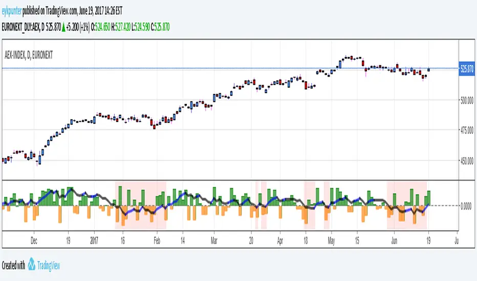
True Balance of powerThis is an improvement of the script published by LazyBear,
The improvements are:
1. it includes gaps because it uses true range in stead of the current bar,
2. it has been turned into a percent oscillator as the basic algorithm belongs in the family of stochastic oscillators.
Unlike the usual stochatics I refrained from over the top averaging and smoothing, nor did I attempt a signal line. There’s no need to make a mock MACD.
The indicator should be interpreted as a stochastics, the difference between Stochs and MACD is that stochs report inclinations, i.e. in which direction the market is edging, while MACD reports movements, in which direction the market is moving. Stochs are an early indicator, MACD is lagging. The emoline is a 30 period linear regression, I use linear regressions because these have no lagging, react immidiately to changes, I use a 30 period version because that is not so nervous. You might say that an MA gives an average while a linear regression gives an ‘over all’ of the periods.
The back ground color is red when the emoline is below zero, that is where the market ‘looks down’, white where the market ‘looks up’. This doesn’t mean that the market will actually go down or up, it may allways change its mind.
Have fun and take care, Eykpunter.
RSI Overbought/Oversold + Divergence Indicator (new)//@version=5
indicator('CryptoSignalScanner - RSI Overbought/Oversold + Divergence Indicator (new)',
//---------------------------------------------------------------------------------------------------------------------------------
//--- Define Colors ---------------------------------------------------------------------------------------------------------------
//---------------------------------------------------------------------------------------------------------------------------------
vWhite = #FFFFFF
vViolet = #C77DF3
vIndigo = #8A2BE2
vBlue = #009CDF
vGreen = #5EBD3E
vYellow = #FFB900
vRed = #E23838
longColor = color.green
shortColor = color.red
textColor = color.white
bullishColor = color.rgb(38,166,154,0) //Used in the display table
bearishColor = color.rgb(239,83,79,0) //Used in the display table
nomatchColor = color.silver //Used in the display table
//---------------------------------------------------------------------------------------------------------------------------------------------------------------------
//--- Functions--------------------------------------------------------------------------------------------------------------------------------------------------------
//---------------------------------------------------------------------------------------------------------------------------------------------------------------------
TF2txt(TF) =>
switch TF
"S" => "RSI 1s:"
"5S" => "RSI 5s:"
"10S" => "RSI 10s:"
"15S" => "RSI 15s:"
"30S" => "RSI 30s"
"1" => "RSI 1m:"
"3" => "RSI 3m:"
"5" => "RSI 5m:"
"15" => "RSI 15m:"
"30" => "RSI 30m"
"45" => "RSI 45m"
"60" => "RSI 1h:"
"120" => "RSI 2h:"
"180" => "RSI 3h:"
"240" => "RSI 4h:"
"480" => "RSI 8h:"
"D" => "RSI 1D:"
"1D" => "RSI 1D:"
"2D" => "RSI 2D:"
"3D" => "RSI 2D:"
"3D" => "RSI 3W:"
"W" => "RSI 1W:"
"1W" => "RSI 1W:"
"M" => "RSI 1M:"
"1M" => "RSI 1M:"
"3M" => "RSI 3M:"
"6M" => "RSI 6M:"
"12M" => "RSI 12M:"
//---------------------------------------------------------------------------------------------------------------------------------------------------------------------
//--- Show/Hide Settings ----------------------------------------------------------------------------------------------------------------------------------------------
//---------------------------------------------------------------------------------------------------------------------------------------------------------------------
rsiShowInput = input(true, title='Show RSI', group='Show/Hide Settings')
maShowInput = input(false, title='Show MA', group='Show/Hide Settings')
showRSIMAInput = input(true, title='Show RSIMA Cloud', group='Show/Hide Settings')
rsiBandShowInput = input(true, title='Show Oversold/Overbought Lines', group='Show/Hide Settings')
rsiBandExtShowInput = input(true, title='Show Oversold/Overbought Extended Lines', group='Show/Hide Settings')
rsiHighlightShowInput = input(true, title='Show Oversold/Overbought Highlight Lines', group='Show/Hide Settings')
DivergenceShowInput = input(true, title='Show RSI Divergence Labels', group='Show/Hide Settings')
//---------------------------------------------------------------------------------------------------------------------------------------------------------------------
//--- Table Settings --------------------------------------------------------------------------------------------------------------------------------------------------
//---------------------------------------------------------------------------------------------------------------------------------------------------------------------
rsiShowTable = input(true, title='Show RSI Table Information box', group="RSI Table Settings")
rsiTablePosition = input.string(title='Location', defval='middle_right', options= , group="RSI Table Settings", inline='1')
rsiTextSize = input.string(title=' Size', defval='small', options= , group="RSI Table Settings", inline='1')
rsiShowTF1 = input(true, title='Show TimeFrame1', group="RSI Table Settings", inline='tf1')
rsiTF1 = input.timeframe("15", title=" Time", group="RSI Table Settings", inline='tf1')
rsiShowTF2 = input(true, title='Show TimeFrame2', group="RSI Table Settings", inline='tf2')
rsiTF2 = input.timeframe("60", title=" Time", group="RSI Table Settings", inline='tf2')
rsiShowTF3 = input(true, title='Show TimeFrame3', group="RSI Table Settings", inline='tf3')
rsiTF3 = input.timeframe("240", title=" Time", group="RSI Table Settings", inline='tf3')
rsiShowTF4 = input(true, title='Show TimeFrame4', group="RSI Table Settings", inline='tf4')
rsiTF4 = input.timeframe("D", title=" Time", group="RSI Table Settings", inline='tf4')
rsiShowHist = input(true, title='Show RSI Historical Columns', group="RSI Table Settings", tooltip='Show the information of the 2 previous closed candles')
//---------------------------------------------------------------------------------------------------------------------------------------------------------------------
//--- RSI Input Settings ----------------------------------------------------------------------------------------------------------------------------------------------
//---------------------------------------------------------------------------------------------------------------------------------------------------------------------
rsiSourceInput = input.source(close, 'Source', group='RSI Settings')
rsiLengthInput = input.int(14, minval=1, title='RSI Length', group='RSI Settings', tooltip='Here we set the RSI lenght')
rsiColorInput = input.color(#26a69a, title="RSI Color", group='RSI Settings')
rsimaColorInput = input.color(#ef534f, title="RSIMA Color", group='RSI Settings')
rsiBandColorInput = input.color(#787B86, title="RSI Band Color", group='RSI Settings')
rsiUpperBandExtInput = input.int(title='RSI Overbought Extended Line', defval=80, minval=50, maxval=100, group='RSI Settings')
rsiUpperBandInput = input.int(title='RSI Overbought Line', defval=70, minval=50, maxval=100, group='RSI Settings')
rsiLowerBandInput = input.int(title='RSI Oversold Line', defval=30, minval=0, maxval=50, group='RSI Settings')
rsiLowerBandExtInput = input.int(title='RSI Oversold Extended Line', defval=20, minval=0, maxval=50, group='RSI Settings')
//---------------------------------------------------------------------------------------------------------------------------------------------------------------------
//--- MA Input Settings -----------------------------------------------------------------------------------------------------------------------------------------------
//---------------------------------------------------------------------------------------------------------------------------------------------------------------------
maTypeInput = input.string("EMA", title="MA Type", options= , group="MA Settings")
maLengthInput = input.int(14, title="MA Length", group="MA Settings")
maColorInput = input.color(color.yellow, title="MA Color", group='MA Settings') //#7E57C2
//---------------------------------------------------------------------------------------------------------------------------------------------------------------------
//--- Divergence Input Settings ---------------------------------------------------------------------------------------------------------------------------------------
//---------------------------------------------------------------------------------------------------------------------------------------------------------------------
lbrInput = input(title="Pivot Lookback Right", defval=2, group='RSI Divergence Settings')
lblInput = input(title="Pivot Lookback Left", defval=2, group='RSI Divergence Settings')
lbRangeMaxInput = input(title="Max of Lookback Range", defval=10, group='RSI Divergence Settings')
lbRangeMinInput = input(title="Min of Lookback Range", defval=2, group='RSI Divergence Settings')
plotBullInput = input(title="Plot Bullish", defval=true, group='RSI Divergence Settings')
plotHiddenBullInput = input(title="Plot Hidden Bullish", defval=true, group='RSI Divergence Settings')
plotBearInput = input(title="Plot Bearish", defval=true, group='RSI Divergence Settings')
plotHiddenBearInput = input(title="Plot Hidden Bearish", defval=true, group='RSI Divergence Settings')
//---------------------------------------------------------------------------------------------------------------------------------------------------------------------
//--- RSI Calculation -------------------------------------------------------------------------------------------------------------------------------------------------
//---------------------------------------------------------------------------------------------------------------------------------------------------------------------
rsi = ta.rsi(rsiSourceInput, rsiLengthInput)
rsiprevious = rsi
= request.security(syminfo.tickerid, rsiTF1, [rsi, rsi , rsi ], lookahead=barmerge.lookahead_on)
= request.security(syminfo.tickerid, rsiTF2, [rsi, rsi , rsi ], lookahead=barmerge.lookahead_on)
= request.security(syminfo.tickerid, rsiTF3, [rsi, rsi , rsi ], lookahead=barmerge.lookahead_on)
= request.security(syminfo.tickerid, rsiTF4, [rsi, rsi , rsi ], lookahead=barmerge.lookahead_on)
//---------------------------------------------------------------------------------------------------------------------------------------------------------------------
//--- MA Calculation -------------------------------------------------------------------------------------------------------------------------------------------------
//---------------------------------------------------------------------------------------------------------------------------------------------------------------------
ma(source, length, type) =>
switch type
"SMA" => ta.sma(source, length)
"Bollinger Bands" => ta.sma(source, length)
"EMA" => ta.ema(source, length)
"SMMA (RMA)" => ta.rma(source, length)
"WMA" => ta.wma(source, length)
"VWMA" => ta.vwma(source, length)
rsiMA = ma(rsi, maLengthInput, maTypeInput)
rsiMAPrevious = rsiMA
//---------------------------------------------------------------------------------------------------------------------------------------------------------------------
//--- Stoch RSI Settings + Calculation --------------------------------------------------------------------------------------------------------------------------------
//---------------------------------------------------------------------------------------------------------------------------------------------------------------------
showStochRSI = input(false, title="Show Stochastic RSI", group='Stochastic RSI Settings')
smoothK = input.int(title="Stochastic K", defval=3, minval=1, maxval=10, group='Stochastic RSI Settings')
smoothD = input.int(title="Stochastic D", defval=4, minval=1, maxval=10, group='Stochastic RSI Settings')
lengthRSI = input.int(title="Stochastic RSI Lenght", defval=14, minval=1, group='Stochastic RSI Settings')
lengthStoch = input.int(title="Stochastic Lenght", defval=14, minval=1, group='Stochastic RSI Settings')
colorK = input.color(color.rgb(41,98,255,0), title="K Color", group='Stochastic RSI Settings', inline="1")
colorD = input.color(color.rgb(205,109,0,0), title="D Color", group='Stochastic RSI Settings', inline="1")
StochRSI = ta.rsi(rsiSourceInput, lengthRSI)
k = ta.sma(ta.stoch(StochRSI, StochRSI, StochRSI, lengthStoch), smoothK) //Blue Line
d = ta.sma(k, smoothD) //Red Line
//---------------------------------------------------------------------------------------------------------------------------------------------------------------------
//--- Divergence Settings ------------------------------------------------------------------------------------------------------------------------------------------
//---------------------------------------------------------------------------------------------------------------------------------------------------------------------
bearColor = color.red
bullColor = color.green
hiddenBullColor = color.new(color.green, 50)
hiddenBearColor = color.new(color.red, 50)
//textColor = color.white
noneColor = color.new(color.white, 100)
osc = rsi
plFound = na(ta.pivotlow(osc, lblInput, lbrInput)) ? false : true
phFound = na(ta.pivothigh(osc, lblInput, lbrInput)) ? false : true
_inRange(cond) =>
bars = ta.barssince(cond == true)
lbRangeMinInput <= bars and bars <= lbRangeMaxInput
//---------------------------------------------------------------------------------------------------------------------------------------------------------------------
//--- Define Plot & Line Colors ---------------------------------------------------------------------------------------------------------------------------------------
//---------------------------------------------------------------------------------------------------------------------------------------------------------------------
rsiColor = rsi >= rsiMA ? rsiColorInput : rsimaColorInput
//---------------------------------------------------------------------------------------------------------------------------------------------------------------------
//--- Plot Lines ------------------------------------------------------------------------------------------------------------------------------------------------------
//---------------------------------------------------------------------------------------------------------------------------------------------------------------------
// Create a horizontal line at a specific price level
myLine = line.new(bar_index , 75, bar_index, 75, color = color.rgb(187, 14, 14), width = 2)
bottom = line.new(bar_index , 50, bar_index, 50, color = color.rgb(223, 226, 28), width = 2)
mymainLine = line.new(bar_index , 60, bar_index, 60, color = color.rgb(13, 154, 10), width = 3)
hline(50, title='RSI Baseline', color=color.new(rsiBandColorInput, 50), linestyle=hline.style_solid, editable=false)
hline(rsiBandExtShowInput ? rsiUpperBandExtInput : na, title='RSI Upper Band', color=color.new(rsiBandColorInput, 10), linestyle=hline.style_dashed, editable=false)
hline(rsiBandShowInput ? rsiUpperBandInput : na, title='RSI Upper Band', color=color.new(rsiBandColorInput, 10), linestyle=hline.style_dashed, editable=false)
hline(rsiBandShowInput ? rsiLowerBandInput : na, title='RSI Upper Band', color=color.new(rsiBandColorInput, 10), linestyle=hline.style_dashed, editable=false)
hline(rsiBandExtShowInput ? rsiLowerBandExtInput : na, title='RSI Upper Band', color=color.new(rsiBandColorInput, 10), linestyle=hline.style_dashed, editable=false)
bgcolor(rsiHighlightShowInput ? rsi >= rsiUpperBandExtInput ? color.new(rsiColorInput, 70) : na : na, title="Show Extended Oversold Highlight", editable=false)
bgcolor(rsiHighlightShowInput ? rsi >= rsiUpperBandInput ? rsi < rsiUpperBandExtInput ? color.new(#64ffda, 90) : na : na: na, title="Show Overbought Highlight", editable=false)
bgcolor(rsiHighlightShowInput ? rsi <= rsiLowerBandInput ? rsi > rsiLowerBandExtInput ? color.new(#F43E32, 90) : na : na : na, title="Show Extended Oversold Highlight", editable=false)
bgcolor(rsiHighlightShowInput ? rsi <= rsiLowerBandInput ? color.new(rsimaColorInput, 70) : na : na, title="Show Oversold Highlight", editable=false)
maPlot = plot(maShowInput ? rsiMA : na, title='MA', color=color.new(maColorInput,0), linewidth=1)
rsiMAPlot = plot(showRSIMAInput ? rsiMA : na, title="RSI EMA", color=color.new(rsimaColorInput,0), editable=false, display=display.none)
rsiPlot = plot(rsiShowInput ? rsi : na, title='RSI', color=color.new(rsiColor,0), linewidth=1)
fill(rsiPlot, rsiMAPlot, color=color.new(rsiColor, 60), title="RSIMA Cloud")
plot(showStochRSI ? k : na, title='Stochastic K', color=colorK, linewidth=1)
plot(showStochRSI ? d : na, title='Stochastic D', color=colorD, linewidth=1)
//---------------------------------------------------------------------------------------------------------------------------------------------------------------------
//--- Plot Divergence -------------------------------------------------------------------------------------------------------------------------------------------------
//---------------------------------------------------------------------------------------------------------------------------------------------------------------------
// Regular Bullish
// Osc: Higher Low
oscHL = osc > ta.valuewhen(plFound, osc , 1) and _inRange(plFound )
// Price: Lower Low
priceLL = low < ta.valuewhen(plFound, low , 1)
bullCond = plotBullInput and priceLL and oscHL and plFound
plot(
plFound ? osc : na,
offset=-lbrInput,
title="Regular Bullish",
linewidth=2,
color=(bullCond ? bullColor : noneColor)
)
plotshape(
DivergenceShowInput ? bullCond ? osc : na : na,
offset=-lbrInput,
title="Regular Bullish Label",
text=" Bull ",
style=shape.labelup,
location=location.absolute,
color=bullColor,
textcolor=textColor
)
//------------------------------------------------------------------------------
// Hidden Bullish
// Osc: Lower Low
oscLL = osc < ta.valuewhen(plFound, osc , 1) and _inRange(plFound )
// Price: Higher Low
priceHL = low > ta.valuewhen(plFound, low , 1)
hiddenBullCond = plotHiddenBullInput and priceHL and oscLL and plFound
plot(
plFound ? osc : na,
offset=-lbrInput,
title="Hidden Bullish",
linewidth=2,
color=(hiddenBullCond ? hiddenBullColor : noneColor)
)
plotshape(
DivergenceShowInput ? hiddenBullCond ? osc : na : na,
offset=-lbrInput,
title="Hidden Bullish Label",
text=" H Bull ",
style=shape.labelup,
location=location.absolute,
color=bullColor,
textcolor=textColor
)
//------------------------------------------------------------------------------
// Regular Bearish
// Osc: Lower High
oscLH = osc < ta.valuewhen(phFound, osc , 1) and _inRange(phFound )
// Price: Higher High
priceHH = high > ta.valuewhen(phFound, high , 1)
bearCond = plotBearInput and priceHH and oscLH and phFound
plot(
phFound ? osc : na,
offset=-lbrInput,
title="Regular Bearish",
linewidth=2,
color=(bearCond ? bearColor : noneColor)
)
plotshape(
DivergenceShowInput ? bearCond ? osc : na : na,
offset=-lbrInput,
title="Regular Bearish Label",
text=" Bear ",
style=shape.labeldown,
location=location.absolute,
color=bearColor,
textcolor=textColor
)
//------------------------------------------------------------------------------
// Hidden Bearish
// Osc: Higher High
oscHH = osc > ta.valuewhen(phFound, osc , 1) and _inRange(phFound )
// Price: Lower High
priceLH = high < ta.valuewhen(phFound, high , 1)
hiddenBearCond = plotHiddenBearInput and priceLH and oscHH and phFound
plot(
phFound ? osc : na,
offset=-lbrInput,
title="Hidden Bearish",
linewidth=2,
color=(hiddenBearCond ? hiddenBearColor : noneColor)
)
plotshape(
DivergenceShowInput ? hiddenBearCond ? osc : na : na,
offset=-lbrInput,
title="Hidden Bearish Label",
text=" H Bear ",
style=shape.labeldown,
location=location.absolute,
color=bearColor,
textcolor=textColor
)
//---------------------------------------------------------------------------------------------------------------------------------------------------------------------
//--- Check RSI Lineup ------------------------------------------------------------------------------------------------------------------------------------------------
//---------------------------------------------------------------------------------------------------------------------------------------------------------------------
bullTF = rsi > rsi and rsi > rsi
bearTF = rsi < rsi and rsi < rsi
bullTF1 = rsi1 > rsi1_1 and rsi1_1 > rsi1_2
bearTF1 = rsi1 < rsi1_1 and rsi1_1 < rsi1_2
bullTF2 = rsi2 > rsi2_1 and rsi2_1 > rsi2_2
bearTF2 = rsi2 < rsi2_1 and rsi2_1 < rsi2_2
bullTF3 = rsi3 > rsi3_1 and rsi3_1 > rsi3_2
bearTF3 = rsi3 < rsi3_1 and rsi3_1 < rsi3_2
bullTF4 = rsi4 > rsi4_1 and rsi4_1 > rsi4_2
bearTF4 = rsi4 < rsi4_1 and rsi4_1 < rsi4_2
bbTxt(bull,bear) =>
bull ? "BULLISH" : bear ? "BEARISCH" : 'NO LINEUP'
bbColor(bull,bear) =>
bull ? bullishColor : bear ? bearishColor : nomatchColor
newTC(tBox, col, row, txt, width, txtColor, bgColor, txtHA, txtSize) =>
table.cell(table_id=tBox,column=col, row=row, text=txt, width=width,text_color=txtColor,bgcolor=bgColor, text_halign=txtHA, text_size=txtSize)
//---------------------------------------------------------------------------------------------------------------------------------------------------------------------
//--- Define RSI Table Setting ----------------------------------------------------------------------------------------------------------------------------------------
//---------------------------------------------------------------------------------------------------------------------------------------------------------------------
width_c0 = 0
width_c1 = 0
if rsiShowTable
var tBox = table.new(position=rsiTablePosition, columns=5, rows=6, bgcolor=color.rgb(18,22,33,50), frame_color=color.black, frame_width=1, border_color=color.black, border_width=1)
newTC(tBox, 0,1,"RSI Current",width_c0,color.orange,color.rgb(0,0,0,100),'right',rsiTextSize)
newTC(tBox, 1,1,str.format(" {0,number,#.##} ", rsi),width_c0,vWhite,rsi < 50 ? bearishColor:bullishColor,'left',rsiTextSize)
newTC(tBox, 4,1,bbTxt(bullTF, bearTF),width_c0,vWhite,bbColor(bullTF, bearTF),'center',rsiTextSize)
if rsiShowHist
newTC(tBox, 2,1,str.format(" {0,number,#.##} ", rsi ),width_c0,vWhite,rsi < 50 ? bearishColor:bullishColor,'left',rsiTextSize)
newTC(tBox, 3,1,str.format(" {0,number,#.##} ", rsi ),width_c0,vWhite,rsi < 50 ? bearishColor:bullishColor,'left',rsiTextSize)
if rsiShowTF1
newTC(tBox, 0,2,TF2txt(rsiTF1),width_c0,vWhite,color.rgb(0,0,0,100),'right',rsiTextSize)
newTC(tBox, 1,2,str.format(" {0,number,#.##} ", rsi1),width_c0,vWhite,rsi1 < 50 ? bearishColor:bullishColor,'left',rsiTextSize)
newTC(tBox, 4,2,bbTxt(bullTF1, bearTF1),width_c0,vWhite,bbColor(bullTF1,bearTF1),'center',rsiTextSize)
if rsiShowHist
newTC(tBox, 2,2,str.format(" {0,number,#.##} ", rsi1_1),width_c0,vWhite,rsi1_1 < 50 ? bearishColor:bullishColor,'left',rsiTextSize)
newTC(tBox, 3,2,str.format(" {0,number,#.##} ", rsi1_2),width_c0,vWhite,rsi1_2 < 50 ? bearishColor:bullishColor,'left',rsiTextSize)
if rsiShowTF2
newTC(tBox, 0,3,TF2txt(rsiTF2),width_c0,vWhite,color.rgb(0,0,0,100),'right',rsiTextSize)
newTC(tBox, 1,3,str.format(" {0,number,#.##} ", rsi2),width_c0,vWhite,rsi2 < 50 ? bearishColor:bullishColor,'left',rsiTextSize)
newTC(tBox, 4,3,bbTxt(bullTF2, bearTF2),width_c0,vWhite,bbColor(bullTF2,bearTF2),'center',rsiTextSize)
if rsiShowHist
newTC(tBox, 2,3,str.format(" {0,number,#.##} ", rsi2_1),width_c0,vWhite,rsi2_1 < 50 ? bearishColor:bullishColor,'left',rsiTextSize)
newTC(tBox, 3,3,str.format(" {0,number,#.##} ", rsi2_2),width_c0,vWhite,rsi2_2 < 50 ? bearishColor:bullishColor,'left',rsiTextSize)
if rsiShowTF3
newTC(tBox, 0,4,TF2txt(rsiTF3),width_c0,vWhite,color.rgb(0,0,0,100),'right',rsiTextSize)
newTC(tBox, 1,4,str.format(" {0,number,#.##} ", rsi3),width_c0,vWhite,rsi3 < 50 ? bearishColor:bullishColor,'left',rsiTextSize)
newTC(tBox, 4,4,bbTxt(bullTF3, bearTF3),width_c0,vWhite,bbColor(bullTF3,bearTF3),'center',rsiTextSize)
if rsiShowHist
newTC(tBox, 2,4,str.format(" {0,number,#.##} ", rsi3_1),width_c0,vWhite,rsi3_1 < 50 ? bearishColor:bullishColor,'left',rsiTextSize)
newTC(tBox, 3,4,str.format(" {0,number,#.##} ", rsi3_2),width_c0,vWhite,rsi3_2 < 50 ? bearishColor:bullishColor,'left',rsiTextSize)
if rsiShowTF4
newTC(tBox, 0,5,TF2txt(rsiTF4),width_c0,vWhite,color.rgb(0,0,0,100),'right',rsiTextSize)
newTC(tBox, 1,5,str.format(" {0,number,#.##} ", rsi4),width_c0,vWhite,rsi4 < 50 ? bearishColor:bullishColor,'left',rsiTextSize)
newTC(tBox, 4,5,bbTxt(bullTF4, bearTF4),width_c0,vWhite,bbColor(bullTF4,bearTF4),'center',rsiTextSize)
if rsiShowHist
newTC(tBox, 2,5,str.format(" {0,number,#.##} ", rsi4_1),width_c0,vWhite,rsi4_1 < 50 ? bearishColor:bullishColor,'left',rsiTextSize)
newTC(tBox, 3,5,str.format(" {0,number,#.##} ", rsi4_2),width_c0,vWhite,rsi4_2 < 50 ? bearishColor:bullishColor,'left',rsiTextSize)
//------------------------------------------------------
//--- Alerts -------------------------------------------
//------------------------------------------------------

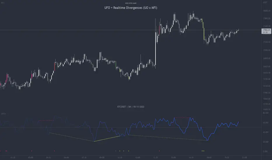
UFO + Realtime Divergences (UO x MFI)UFO + Realtime Divergences (UO x MFI) + Alerts
The UFO is a hybrid of two powerful oscillators - the Ultimate Oscillator (UO) and the Money Flow Index (MFI)
Features of the UFO include:
- Optional divergence lines drawn directly onto the oscillator in realtime.
- Configurable alerts to notify you when divergences occur, as well as centerline crossovers.
- Configurable lookback periods to fine tune the divergences drawn in order to suit different trading styles and timeframes.
- Background colouring option to indicate when the oscillator has crossed its centerline.
- Alternate timeframe feature allows you to configure the oscillator to use data from a different timeframe than the chart it is loaded on.
- 2x MTF triple-timeframe Stochastic RSI overbought and oversold confluence signals painted at the top of the panel for use as a confluence for reversal entry trades.
The core calculations of the UFO+ combine the factory settings of the Ultimate Oscillator and Money Flow Index, taking an average of their combined values for its output eg:
UO_Value + MFI_Value / 2
The result is a powerful oscillator capable of detecting high quality divergences, including on very low timeframes and highly volatile markets, it benefits from the higher weighting of the most recent price action provided by the Ultimate Oscillators calculations, as well as the calculation of the MFI, which incorporates volume data. The UFO and its incorporated 2x triple-timeframe MTF Stoch RSI overbought and oversold signals makes it well adapted for low timeframe scalping and regular divergence trades in particular.
The Ultimate Oscillator (UO)
Tradingview describes the Ultimate Oscillator as follows:
“The Ultimate Oscillator indicator (UO) is a technical analysis tool used to measure momentum across three varying timeframes. The problem with many momentum oscillators is that after a rapid advance or decline in price, they can form false divergence trading signals. For example, after a rapid rise in price, a bearish divergence signal may present itself, however price continues to rise. The Ultimate Oscillator attempts to correct this by using multiple timeframes in its calculation as opposed to just one timeframe which is what is used in most other momentum oscillators.”
You can read more about the UO and its calculations here
The Money Flow Index ( MFI )
Investopedia describes the True Strength Indicator as follows:
“The Money Flow Index ( MFI ) is a technical oscillator that uses price and volume data for identifying overbought or oversold signals in an asset. It can also be used to spot divergences which warn of a trend change in price. The oscillator moves between 0 and 100. Unlike conventional oscillators such as the Relative Strength Index ( RSI ), the Money Flow Index incorporates both price and volume data, as opposed to just price. For this reason, some analysts call MFI the volume-weighted RSI .”
You can read more about the MFI and its calculations here
The Stochastic RSI (relating to the built-in MTF Stoch RSI feature)
The popular oscillator has been described as follows:
“The Stochastic RSI is an indicator used in technical analysis that ranges between zero and one (or zero and 100 on some charting platforms) and is created by applying the Stochastic oscillator formula to a set of relative strength index ( RSI ) values rather than to standard price data. Using RSI values within the Stochastic formula gives traders an idea of whether the current RSI value is overbought or oversold. The Stochastic RSI oscillator was developed to take advantage of both momentum indicators in order to create a more sensitive indicator that is attuned to a specific security's historical performance rather than a generalized analysis of price change.”
You can read more about the Stochastic RSI and its calculations here
How do traders use overbought and oversold levels in their trading?
The oversold level, that is when the Stochastic RSI is above the 80 level is typically interpreted as being 'overbought', and below the 20 level is typically considered 'oversold'. Traders will often use the Stochastic RSI at an overbought level as a confluence for entry into a short position, and the Stochastic RSI at an oversold level as a confluence for an entry into a long position. These levels do not mean that price will necessarily reverse at those levels in a reliable way, however. This is why this version of the Stoch RSI employs the triple timeframe overbought and oversold confluence, in an attempt to add a more confluence and reliability to this usage of the Stoch RSI .
What are divergences?
Divergence is when the price of an asset is moving in the opposite direction of a technical indicator, such as an oscillator, or is moving contrary to other data. Divergence warns that the current price trend may be weakening, and in some cases may lead to the price changing direction.
There are 4 main types of divergence, which are split into 2 categories;
regular divergences and hidden divergences. Regular divergences indicate possible trend reversals, and hidden divergences indicate possible trend continuation.
Regular bullish divergence: An indication of a potential trend reversal, from the current downtrend, to an uptrend.
Regular bearish divergence: An indication of a potential trend reversal, from the current uptrend, to a downtrend.
Hidden bullish divergence: An indication of a potential uptrend continuation.
Hidden bearish divergence: An indication of a potential downtrend continuation.
How do traders use divergences in their trading?
A divergence is considered a leading indicator in technical analysis , meaning it has the ability to indicate a potential price move in the short term future.
Hidden bullish and hidden bearish divergences, which indicate a potential continuation of the current trend are sometimes considered a good place for traders to begin, since trend continuation occurs more frequently than reversals, or trend changes.
When trading regular bullish divergences and regular bearish divergences, which are indications of a trend reversal, the probability of it doing so may increase when these occur at a strong support or resistance level . A common mistake new traders make is to get into a regular divergence trade too early, assuming it will immediately reverse, but these can continue to form for some time before the trend eventually changes, by using forms of support or resistance as an added confluence, such as when price reaches a moving average, the success rate when trading these patterns may increase.
Typically, traders will manually draw lines across the swing highs and swing lows of both the price chart and the oscillator to see whether they appear to present a divergence, this indicator will draw them for you, quickly and clearly, and can notify you when they occur.
Setting alerts.
With this indicator you can set alerts to notify you when any/all of the above types of divergences occur, on any chart timeframe you choose.
Configurable pivot period.
You can adjust the default pivot lookback values to suit your prefered trading style and timeframe. If you like to trade a shorter time frame, lowering the default lookback values will make the divergences drawn more sensitive to short term price action.
Disclaimer: This script includes code from the stock UO and MFI by Tradingview as well as the Divergence for Many Indicators v4 by LonesomeTheBlue.
Multi EMA + Indicators + Mini-Dashboard + Reversals v6📘 Multi EMA + Indicators + Mini-Dashboard + Reversals v6
🧩 Overview
This indicator is a multi-EMA setup that combines trend, momentum, and reversal analysis in a single visual framework.
It integrates four exponential moving averages (EMAs), key oscillators (RSI, MACD, Stochastic, CCI), volatility filtering (ATR), and a dynamic mini-dashboard that summarizes all signals in real time.
Its purpose is to help traders visually confirm trend alignment, filter valid entries, and identify possible trend continuation or reversal points.
It can display buy/sell arrows, detect reversal candles, and issue alerts when trading conditions are met.
⚙️ Core Components
1. Moving Averages (EMA Setup)
EMA1 (fast) and EMA2 (medium) define the short-term trend and trigger bias.
When the price is above both EMAs → bullish bias.
When below → bearish bias.
EMA3 and EMA4 act as trend filters. Their slopes (up or down) confirm overall momentum and help validate signals.
Each EMA has customizable lengths, sources, and colors for up/down trends.
This “EMA stack” is the foundation of the setup — a structured trend-following framework that adapts to market speed and volatility.
2. Momentum and Confirmation Filters
Each indicator can be individually enabled or disabled for flexibility.
RSI: confirms direction (above/below 50).
MACD: detects momentum crossover (MACD > Signal for bullish confirmation).
Stochastic: identifies trend continuation (K > D for longs, K < D for shorts).
CCI: adds trend bias above/below a threshold.
ATR Filter: filters out small, low-volatility candles to reduce noise.
You can activate only the filters that fit your trading plan — for instance, trend traders often use RSI and MACD, while scalpers may rely on Stochastic and ATR.
3. Reversal Detection
The indicator includes an optional Reversal Section that independently detects potential turning points.
It combines multiple configurable criteria:
Candlestick patterns (Bullish Hammer, Shooting Star).
Large Candle filter — detects unusually large bars (relative to close).
Price-to-EMA distance — identifies overextended moves that might revert.
RSI Divergence — detects potential momentum shifts.
RSI Overbought/Oversold zones (70/30 by default).
Doji Candles — sign of indecision.
A bullish or bearish reversal signal appears when enough selected criteria are met.
All sub-modules can be toggled on/off individually, giving you full control over sensitivity.
4. Signal Logic
Buy and sell signals are triggered when EMA alignment and the chosen confirmations agree:
Buy Signal
→ Price above EMA1 & EMA2
→ Confirmations (RSI/MACD/Stoch/CCI/ATR) pass
→ Trend filters (EMA3/EMA4) point upward
Sell Signal
→ Price below EMA1 & EMA2
→ Confirmations align bearishly
→ Trend filters (EMA3/EMA4) slope downward
Reversal signals can appear independently, even against the current EMA trend, depending on your settings.
5. Visual Dashboard
A mini-dashboard appears near the chart showing:
Current trade bias (LONG / SHORT / NEUTRAL)
EMA3 and EMA4 trend directions (↑ / ↓)
Quick visual bars (🟩 / 🟥) for each filter: RSI, MACD, Stoch, ATR, CCI, EMA filters
Reversal criteria status (Doji, RSI divergence, candle size, etc.)
This panel gives you a compact overview of all indicator states at a glance.
The color of the panel changes dynamically — green for bullish, red for bearish, gray for neutral.
6. Alerts
Built-in alerts allow automation or notifications:
Buy Alert
Sell Alert
Reversal Buy
Reversal Sell
You can connect these alerts to TradingView notifications or external bots for semi-automated execution.
💡 How to Use
✅ Trend-Following Setup
Focus on trades in the direction of EMA1 & EMA2.
Confirm with EMA3 & EMA4 trending in the same direction.
Use RSI/MACD/Stoch filters to ensure momentum supports the trade.
Avoid entries when ATR filter indicates low volatility.
🔄 Reversal Setup
Enable the Reversal section for potential tops/bottoms.
Look for reversal buy signals near support zones or after strong downtrends.
Use RSI divergence or Doji + Hammer signals as confirmation.
Combine with key chart areas (supply/demand or previous swing levels).
⚖️ Combination Approach
Trade continuation signals when all EMAs are aligned and filters are green.
Trade reversals only when at a key area (support/resistance) and confirmed by reversal conditions.
Always check higher-timeframe bias before entering a trade.
🧭 Practical Tips
Use different EMA sets for different timeframes:
9/21/50/100 for swing or trend trades.
5/13/34/89 for intraday scalping.
Turn off filters you don’t use to reduce lag.
Always validate signals with price structure, not just indicator alignment.
Practice in replay mode before live trading.
🗺️ Key Chart Confluence (Highly Recommended)
Although the indicator provides structured signals, its best use is in confluence with:
Support and resistance levels
Supply/demand zones
Trendlines and channels
Liquidity pools
Volume clusters
Signals aligned with strong key areas on the chart tend to have greater reliability than isolated indicator triggers.
I use EMA 1 - 20 Open ; EMA 2 - 20 Close ; EMA 3 - 50 ; EMA 4 - 200 or 100 , but that's me...
⚠️ Important Disclaimer
This indicator is a technical tool, not a guarantee of results.
Trading involves risk, and no signal is ever 100% accurate.
Every trader should develop a personal strategy, use proper risk management, and adapt settings to their instrument and timeframe.
Always combine indicator signals with key chart areas, higher-timeframe context, and your own analysis before taking a trade.

Quantum Rotational Field MappingQuantum Rotational Field Mapping (QRFM):
Phase Coherence Detection Through Complex-Plane Oscillator Analysis
Quantum Rotational Field Mapping applies complex-plane mathematics and phase-space analysis to oscillator ensembles, identifying high-probability trend ignition points by measuring when multiple independent oscillators achieve phase coherence. Unlike traditional multi-oscillator approaches that simply stack indicators or use boolean AND/OR logic, this system converts each oscillator into a rotating phasor (vector) in the complex plane and calculates the Coherence Index (CI) —a mathematical measure of how tightly aligned the ensemble has become—then generates signals only when alignment, phase direction, and pairwise entanglement all converge.
The indicator combines three mathematical frameworks: phasor representation using analytic signal theory to extract phase and amplitude from each oscillator, coherence measurement using vector summation in the complex plane to quantify group alignment, and entanglement analysis that calculates pairwise phase agreement across all oscillator combinations. This creates a multi-dimensional confirmation system that distinguishes between random oscillator noise and genuine regime transitions.
What Makes This Original
Complex-Plane Phasor Framework
This indicator implements classical signal processing mathematics adapted for market oscillators. Each oscillator—whether RSI, MACD, Stochastic, CCI, Williams %R, MFI, ROC, or TSI—is first normalized to a common scale, then converted into a complex-plane representation using an in-phase (I) and quadrature (Q) component. The in-phase component is the oscillator value itself, while the quadrature component is calculated as the first difference (derivative proxy), creating a velocity-aware representation.
From these components, the system extracts:
Phase (φ) : Calculated as φ = atan2(Q, I), representing the oscillator's position in its cycle (mapped to -180° to +180°)
Amplitude (A) : Calculated as A = √(I² + Q²), representing the oscillator's strength or conviction
This mathematical approach is fundamentally different from simply reading oscillator values. A phasor captures both where an oscillator is in its cycle (phase angle) and how strongly it's expressing that position (amplitude). Two oscillators can have the same value but be in opposite phases of their cycles—traditional analysis would see them as identical, while QRFM sees them as 180° out of phase (contradictory).
Coherence Index Calculation
The core innovation is the Coherence Index (CI) , borrowed from physics and signal processing. When you have N oscillators, each with phase φₙ, you can represent each as a unit vector in the complex plane: e^(iφₙ) = cos(φₙ) + i·sin(φₙ).
The CI measures what happens when you sum all these vectors:
Resultant Vector : R = Σ e^(iφₙ) = Σ cos(φₙ) + i·Σ sin(φₙ)
Coherence Index : CI = |R| / N
Where |R| is the magnitude of the resultant vector and N is the number of active oscillators.
The CI ranges from 0 to 1:
CI = 1.0 : Perfect coherence—all oscillators have identical phase angles, vectors point in the same direction, creating maximum constructive interference
CI = 0.0 : Complete decoherence—oscillators are randomly distributed around the circle, vectors cancel out through destructive interference
0 < CI < 1 : Partial alignment—some clustering with some scatter
This is not a simple average or correlation. The CI captures phase synchronization across the entire ensemble simultaneously. When oscillators phase-lock (align their cycles), the CI spikes regardless of their individual values. This makes it sensitive to regime transitions that traditional indicators miss.
Dominant Phase and Direction Detection
Beyond measuring alignment strength, the system calculates the dominant phase of the ensemble—the direction the resultant vector points:
Dominant Phase : φ_dom = atan2(Σ sin(φₙ), Σ cos(φₙ))
This gives the "average direction" of all oscillator phases, mapped to -180° to +180°:
+90° to -90° (right half-plane): Bullish phase dominance
+90° to +180° or -90° to -180° (left half-plane): Bearish phase dominance
The combination of CI magnitude (coherence strength) and dominant phase angle (directional bias) creates a two-dimensional signal space. High CI alone is insufficient—you need high CI plus dominant phase pointing in a tradeable direction. This dual requirement is what separates QRFM from simple oscillator averaging.
Entanglement Matrix and Pairwise Coherence
While the CI measures global alignment, the entanglement matrix measures local pairwise relationships. For every pair of oscillators (i, j), the system calculates:
E(i,j) = |cos(φᵢ - φⱼ)|
This represents the phase agreement between oscillators i and j:
E = 1.0 : Oscillators are in-phase (0° or 360° apart)
E = 0.0 : Oscillators are in quadrature (90° apart, orthogonal)
E between 0 and 1 : Varying degrees of alignment
The system counts how many oscillator pairs exceed a user-defined entanglement threshold (e.g., 0.7). This entangled pairs count serves as a confirmation filter: signals require not just high global CI, but also a minimum number of strong pairwise agreements. This prevents false ignitions where CI is high but driven by only two oscillators while the rest remain scattered.
The entanglement matrix creates an N×N symmetric matrix that can be visualized as a web—when many cells are bright (high E values), the ensemble is highly interconnected. When cells are dark, oscillators are moving independently.
Phase-Lock Tolerance Mechanism
A complementary confirmation layer is the phase-lock detector . This calculates the maximum phase spread across all oscillators:
For all pairs (i,j), compute angular distance: Δφ = |φᵢ - φⱼ|, wrapping at 180°
Max Spread = maximum Δφ across all pairs
If max spread < user threshold (e.g., 35°), the ensemble is considered phase-locked —all oscillators are within a narrow angular band.
This differs from entanglement: entanglement measures pairwise cosine similarity (magnitude of alignment), while phase-lock measures maximum angular deviation (tightness of clustering). Both must be satisfied for the highest-conviction signals.
Multi-Layer Visual Architecture
QRFM includes six visual components that represent the same underlying mathematics from different perspectives:
Circular Orbit Plot : A polar coordinate grid showing each oscillator as a vector from origin to perimeter. Angle = phase, radius = amplitude. This is a real-time snapshot of the complex plane. When vectors converge (point in similar directions), coherence is high. When scattered randomly, coherence is low. Users can see phase alignment forming before CI numerically confirms it.
Phase-Time Heat Map : A 2D matrix with rows = oscillators and columns = time bins. Each cell is colored by the oscillator's phase at that time (using a gradient where color hue maps to angle). Horizontal color bands indicate sustained phase alignment over time. Vertical color bands show moments when all oscillators shared the same phase (ignition points). This provides historical pattern recognition.
Entanglement Web Matrix : An N×N grid showing E(i,j) for all pairs. Cells are colored by entanglement strength—bright yellow/gold for high E, dark gray for low E. This reveals which oscillators are driving coherence and which are lagging. For example, if RSI and MACD show high E but Stochastic shows low E with everything, Stochastic is the outlier.
Quantum Field Cloud : A background color overlay on the price chart. Color (green = bullish, red = bearish) is determined by dominant phase. Opacity is determined by CI—high CI creates dense, opaque cloud; low CI creates faint, nearly invisible cloud. This gives an atmospheric "feel" for regime strength without looking at numbers.
Phase Spiral : A smoothed plot of dominant phase over recent history, displayed as a curve that wraps around price. When the spiral is tight and rotating steadily, the ensemble is in coherent rotation (trending). When the spiral is loose or erratic, coherence is breaking down.
Dashboard : A table showing real-time metrics: CI (as percentage), dominant phase (in degrees with directional arrow), field strength (CI × average amplitude), entangled pairs count, phase-lock status (locked/unlocked), quantum state classification ("Ignition", "Coherent", "Collapse", "Chaos"), and collapse risk (recent CI change normalized to 0-100%).
Each component is independently toggleable, allowing users to customize their workspace. The orbit plot is the most essential—it provides intuitive, visual feedback on phase alignment that no numerical dashboard can match.
Core Components and How They Work Together
1. Oscillator Normalization Engine
The foundation is creating a common measurement scale. QRFM supports eight oscillators:
RSI : Normalized from to using overbought/oversold levels (70, 30) as anchors
MACD Histogram : Normalized by dividing by rolling standard deviation, then clamped to
Stochastic %K : Normalized from using (80, 20) anchors
CCI : Divided by 200 (typical extreme level), clamped to
Williams %R : Normalized from using (-20, -80) anchors
MFI : Normalized from using (80, 20) anchors
ROC : Divided by 10, clamped to
TSI : Divided by 50, clamped to
Each oscillator can be individually enabled/disabled. Only active oscillators contribute to phase calculations. The normalization removes scale differences—a reading of +0.8 means "strongly bullish" regardless of whether it came from RSI or TSI.
2. Analytic Signal Construction
For each active oscillator at each bar, the system constructs the analytic signal:
In-Phase (I) : The normalized oscillator value itself
Quadrature (Q) : The bar-to-bar change in the normalized value (first derivative approximation)
This creates a 2D representation: (I, Q). The phase is extracted as:
φ = atan2(Q, I) × (180 / π)
This maps the oscillator to a point on the unit circle. An oscillator at the same value but rising (positive Q) will have a different phase than one that is falling (negative Q). This velocity-awareness is critical—it distinguishes between "at resistance and stalling" versus "at resistance and breaking through."
The amplitude is extracted as:
A = √(I² + Q²)
This represents the distance from origin in the (I, Q) plane. High amplitude means the oscillator is far from neutral (strong conviction). Low amplitude means it's near zero (weak/transitional state).
3. Coherence Calculation Pipeline
For each bar (or every Nth bar if phase sample rate > 1 for performance):
Step 1 : Extract phase φₙ for each of the N active oscillators
Step 2 : Compute complex exponentials: Zₙ = e^(i·φₙ·π/180) = cos(φₙ·π/180) + i·sin(φₙ·π/180)
Step 3 : Sum the complex exponentials: R = Σ Zₙ = (Σ cos φₙ) + i·(Σ sin φₙ)
Step 4 : Calculate magnitude: |R| = √
Step 5 : Normalize by count: CI_raw = |R| / N
Step 6 : Smooth the CI: CI = SMA(CI_raw, smoothing_window)
The smoothing step (default 2 bars) removes single-bar noise spikes while preserving structural coherence changes. Users can adjust this to control reactivity versus stability.
The dominant phase is calculated as:
φ_dom = atan2(Σ sin φₙ, Σ cos φₙ) × (180 / π)
This is the angle of the resultant vector R in the complex plane.
4. Entanglement Matrix Construction
For all unique pairs of oscillators (i, j) where i < j:
Step 1 : Get phases φᵢ and φⱼ
Step 2 : Compute phase difference: Δφ = φᵢ - φⱼ (in radians)
Step 3 : Calculate entanglement: E(i,j) = |cos(Δφ)|
Step 4 : Store in symmetric matrix: matrix = matrix = E(i,j)
The matrix is then scanned: count how many E(i,j) values exceed the user-defined threshold (default 0.7). This count is the entangled pairs metric.
For visualization, the matrix is rendered as an N×N table where cell brightness maps to E(i,j) intensity.
5. Phase-Lock Detection
Step 1 : For all unique pairs (i, j), compute angular distance: Δφ = |φᵢ - φⱼ|
Step 2 : Wrap angles: if Δφ > 180°, set Δφ = 360° - Δφ
Step 3 : Find maximum: max_spread = max(Δφ) across all pairs
Step 4 : Compare to tolerance: phase_locked = (max_spread < tolerance)
If phase_locked is true, all oscillators are within the specified angular cone (e.g., 35°). This is a boolean confirmation filter.
6. Signal Generation Logic
Signals are generated through multi-layer confirmation:
Long Ignition Signal :
CI crosses above ignition threshold (e.g., 0.80)
AND dominant phase is in bullish range (-90° < φ_dom < +90°)
AND phase_locked = true
AND entangled_pairs >= minimum threshold (e.g., 4)
Short Ignition Signal :
CI crosses above ignition threshold
AND dominant phase is in bearish range (φ_dom < -90° OR φ_dom > +90°)
AND phase_locked = true
AND entangled_pairs >= minimum threshold
Collapse Signal :
CI at bar minus CI at current bar > collapse threshold (e.g., 0.55)
AND CI at bar was above 0.6 (must collapse from coherent state, not from already-low state)
These are strict conditions. A high CI alone does not generate a signal—dominant phase must align with direction, oscillators must be phase-locked, and sufficient pairwise entanglement must exist. This multi-factor gating dramatically reduces false signals compared to single-condition triggers.
Calculation Methodology
Phase 1: Oscillator Computation and Normalization
On each bar, the system calculates the raw values for all enabled oscillators using standard Pine Script functions:
RSI: ta.rsi(close, length)
MACD: ta.macd() returning histogram component
Stochastic: ta.stoch() smoothed with ta.sma()
CCI: ta.cci(close, length)
Williams %R: ta.wpr(length)
MFI: ta.mfi(hlc3, length)
ROC: ta.roc(close, length)
TSI: ta.tsi(close, short, long)
Each raw value is then passed through a normalization function:
normalize(value, overbought_level, oversold_level) = 2 × (value - oversold) / (overbought - oversold) - 1
This maps the oscillator's typical range to , where -1 represents extreme bearish, 0 represents neutral, and +1 represents extreme bullish.
For oscillators without fixed ranges (MACD, ROC, TSI), statistical normalization is used: divide by a rolling standard deviation or fixed divisor, then clamp to .
Phase 2: Phasor Extraction
For each normalized oscillator value val:
I = val (in-phase component)
Q = val - val (quadrature component, first difference)
Phase calculation:
phi_rad = atan2(Q, I)
phi_deg = phi_rad × (180 / π)
Amplitude calculation:
A = √(I² + Q²)
These values are stored in arrays: osc_phases and osc_amps for each oscillator n.
Phase 3: Complex Summation and Coherence
Initialize accumulators:
sum_cos = 0
sum_sin = 0
For each oscillator n = 0 to N-1:
phi_rad = osc_phases × (π / 180)
sum_cos += cos(phi_rad)
sum_sin += sin(phi_rad)
Resultant magnitude:
resultant_mag = √(sum_cos² + sum_sin²)
Coherence Index (raw):
CI_raw = resultant_mag / N
Smoothed CI:
CI = SMA(CI_raw, smoothing_window)
Dominant phase:
phi_dom_rad = atan2(sum_sin, sum_cos)
phi_dom_deg = phi_dom_rad × (180 / π)
Phase 4: Entanglement Matrix Population
For i = 0 to N-2:
For j = i+1 to N-1:
phi_i = osc_phases × (π / 180)
phi_j = osc_phases × (π / 180)
delta_phi = phi_i - phi_j
E = |cos(delta_phi)|
matrix_index_ij = i × N + j
matrix_index_ji = j × N + i
entangle_matrix = E
entangle_matrix = E
if E >= threshold:
entangled_pairs += 1
The matrix uses flat array storage with index mapping: index(row, col) = row × N + col.
Phase 5: Phase-Lock Check
max_spread = 0
For i = 0 to N-2:
For j = i+1 to N-1:
delta = |osc_phases - osc_phases |
if delta > 180:
delta = 360 - delta
max_spread = max(max_spread, delta)
phase_locked = (max_spread < tolerance)
Phase 6: Signal Evaluation
Ignition Long :
ignition_long = (CI crosses above threshold) AND
(phi_dom > -90 AND phi_dom < 90) AND
phase_locked AND
(entangled_pairs >= minimum)
Ignition Short :
ignition_short = (CI crosses above threshold) AND
(phi_dom < -90 OR phi_dom > 90) AND
phase_locked AND
(entangled_pairs >= minimum)
Collapse :
CI_prev = CI
collapse = (CI_prev - CI > collapse_threshold) AND (CI_prev > 0.6)
All signals are evaluated on bar close. The crossover and crossunder functions ensure signals fire only once when conditions transition from false to true.
Phase 7: Field Strength and Visualization Metrics
Average Amplitude :
avg_amp = (Σ osc_amps ) / N
Field Strength :
field_strength = CI × avg_amp
Collapse Risk (for dashboard):
collapse_risk = (CI - CI) / max(CI , 0.1)
collapse_risk_pct = clamp(collapse_risk × 100, 0, 100)
Quantum State Classification :
if (CI > threshold AND phase_locked):
state = "Ignition"
else if (CI > 0.6):
state = "Coherent"
else if (collapse):
state = "Collapse"
else:
state = "Chaos"
Phase 8: Visual Rendering
Orbit Plot : For each oscillator, convert polar (phase, amplitude) to Cartesian (x, y) for grid placement:
radius = amplitude × grid_center × 0.8
x = radius × cos(phase × π/180)
y = radius × sin(phase × π/180)
col = center + x (mapped to grid coordinates)
row = center - y
Heat Map : For each oscillator row and time column, retrieve historical phase value at lookback = (columns - col) × sample_rate, then map phase to color using a hue gradient.
Entanglement Web : Render matrix as table cell with background color opacity = E(i,j).
Field Cloud : Background color = (phi_dom > -90 AND phi_dom < 90) ? green : red, with opacity = mix(min_opacity, max_opacity, CI).
All visual components render only on the last bar (barstate.islast) to minimize computational overhead.
How to Use This Indicator
Step 1 : Apply QRFM to your chart. It works on all timeframes and asset classes, though 15-minute to 4-hour timeframes provide the best balance of responsiveness and noise reduction.
Step 2 : Enable the dashboard (default: top right) and the circular orbit plot (default: middle left). These are your primary visual feedback tools.
Step 3 : Optionally enable the heat map, entanglement web, and field cloud based on your preference. New users may find all visuals overwhelming; start with dashboard + orbit plot.
Step 4 : Observe for 50-100 bars to let the indicator establish baseline coherence patterns. Markets have different "normal" CI ranges—some instruments naturally run higher or lower coherence.
Understanding the Circular Orbit Plot
The orbit plot is a polar grid showing oscillator vectors in real-time:
Center point : Neutral (zero phase and amplitude)
Each vector : A line from center to a point on the grid
Vector angle : The oscillator's phase (0° = right/east, 90° = up/north, 180° = left/west, -90° = down/south)
Vector length : The oscillator's amplitude (short = weak signal, long = strong signal)
Vector label : First letter of oscillator name (R = RSI, M = MACD, etc.)
What to watch :
Convergence : When all vectors cluster in one quadrant or sector, CI is rising and coherence is forming. This is your pre-signal warning.
Scatter : When vectors point in random directions (360° spread), CI is low and the market is in a non-trending or transitional regime.
Rotation : When the cluster rotates smoothly around the circle, the ensemble is in coherent oscillation—typically seen during steady trends.
Sudden flips : When the cluster rapidly jumps from one side to the opposite (e.g., +90° to -90°), a phase reversal has occurred—often coinciding with trend reversals.
Example: If you see RSI, MACD, and Stochastic all pointing toward 45° (northeast) with long vectors, while CCI, TSI, and ROC point toward 40-50° as well, coherence is high and dominant phase is bullish. Expect an ignition signal if CI crosses threshold.
Reading Dashboard Metrics
The dashboard provides numerical confirmation of what the orbit plot shows visually:
CI : Displays as 0-100%. Above 70% = high coherence (strong regime), 40-70% = moderate, below 40% = low (poor conditions for trend entries).
Dom Phase : Angle in degrees with directional arrow. ⬆ = bullish bias, ⬇ = bearish bias, ⬌ = neutral.
Field Strength : CI weighted by amplitude. High values (> 0.6) indicate not just alignment but strong alignment.
Entangled Pairs : Count of oscillator pairs with E > threshold. Higher = more confirmation. If minimum is set to 4, you need at least 4 pairs entangled for signals.
Phase Lock : 🔒 YES (all oscillators within tolerance) or 🔓 NO (spread too wide).
State : Real-time classification:
🚀 IGNITION: CI just crossed threshold with phase-lock
⚡ COHERENT: CI is high and stable
💥 COLLAPSE: CI has dropped sharply
🌀 CHAOS: Low CI, scattered phases
Collapse Risk : 0-100% scale based on recent CI change. Above 50% warns of imminent breakdown.
Interpreting Signals
Long Ignition (Blue Triangle Below Price) :
Occurs when CI crosses above threshold (e.g., 0.80)
Dominant phase is in bullish range (-90° to +90°)
All oscillators are phase-locked (within tolerance)
Minimum entangled pairs requirement met
Interpretation : The oscillator ensemble has transitioned from disorder to coherent bullish alignment. This is a high-probability long entry point. The multi-layer confirmation (CI + phase direction + lock + entanglement) ensures this is not a single-oscillator whipsaw.
Short Ignition (Red Triangle Above Price) :
Same conditions as long, but dominant phase is in bearish range (< -90° or > +90°)
Interpretation : Coherent bearish alignment has formed. High-probability short entry.
Collapse (Circles Above and Below Price) :
CI has dropped by more than the collapse threshold (e.g., 0.55) over a 5-bar window
CI was previously above 0.6 (collapsing from coherent state)
Interpretation : Phase coherence has broken down. If you are in a position, this is an exit warning. If looking to enter, stand aside—regime is transitioning.
Phase-Time Heat Map Patterns
Enable the heat map and position it at bottom right. The rows represent individual oscillators, columns represent time bins (most recent on left).
Pattern: Horizontal Color Bands
If a row (e.g., RSI) shows consistent color across columns (say, green for several bins), that oscillator has maintained stable phase over time. If all rows show horizontal bands of similar color, the entire ensemble has been phase-locked for an extended period—this is a strong trending regime.
Pattern: Vertical Color Bands
If a column (single time bin) shows all cells with the same or very similar color, that moment in time had high coherence. These vertical bands often align with ignition signals or major price pivots.
Pattern: Rainbow Chaos
If cells are random colors (red, green, yellow mixed with no pattern), coherence is low. The ensemble is scattered. Avoid trading during these periods unless you have external confirmation.
Pattern: Color Transition
If you see a row transition from red to green (or vice versa) sharply, that oscillator has phase-flipped. If multiple rows do this simultaneously, a regime change is underway.
Entanglement Web Analysis
Enable the web matrix (default: opposite corner from heat map). It shows an N×N grid where N = number of active oscillators.
Bright Yellow/Gold Cells : High pairwise entanglement. For example, if the RSI-MACD cell is bright gold, those two oscillators are moving in phase. If the RSI-Stochastic cell is bright, they are entangled as well.
Dark Gray Cells : Low entanglement. Oscillators are decorrelated or in quadrature.
Diagonal : Always marked with "—" because an oscillator is always perfectly entangled with itself.
How to use :
Scan for clustering: If most cells are bright, coherence is high across the board. If only a few cells are bright, coherence is driven by a subset (e.g., RSI and MACD are aligned, but nothing else is—weak signal).
Identify laggards: If one row/column is entirely dark, that oscillator is the outlier. You may choose to disable it or monitor for when it joins the group (late confirmation).
Watch for web formation: During low-coherence periods, the matrix is mostly dark. As coherence builds, cells begin lighting up. A sudden "web" of connections forming visually precedes ignition signals.
Trading Workflow
Step 1: Monitor Coherence Level
Check the dashboard CI metric or observe the orbit plot. If CI is below 40% and vectors are scattered, conditions are poor for trend entries. Wait.
Step 2: Detect Coherence Building
When CI begins rising (say, from 30% to 50-60%) and you notice vectors on the orbit plot starting to cluster, coherence is forming. This is your alert phase—do not enter yet, but prepare.
Step 3: Confirm Phase Direction
Check the dominant phase angle and the orbit plot quadrant where clustering is occurring:
Clustering in right half (0° to ±90°): Bullish bias forming
Clustering in left half (±90° to 180°): Bearish bias forming
Verify the dashboard shows the corresponding directional arrow (⬆ or ⬇).
Step 4: Wait for Signal Confirmation
Do not enter based on rising CI alone. Wait for the full ignition signal:
CI crosses above threshold
Phase-lock indicator shows 🔒 YES
Entangled pairs count >= minimum
Directional triangle appears on chart
This ensures all layers have aligned.
Step 5: Execute Entry
Long : Blue triangle below price appears → enter long
Short : Red triangle above price appears → enter short
Step 6: Position Management
Initial Stop : Place stop loss based on your risk management rules (e.g., recent swing low/high, ATR-based buffer).
Monitoring :
Watch the field cloud density. If it remains opaque and colored in your direction, the regime is intact.
Check dashboard collapse risk. If it rises above 50%, prepare for exit.
Monitor the orbit plot. If vectors begin scattering or the cluster flips to the opposite side, coherence is breaking.
Exit Triggers :
Collapse signal fires (circles appear)
Dominant phase flips to opposite half-plane
CI drops below 40% (coherence lost)
Price hits your profit target or trailing stop
Step 7: Post-Exit Analysis
After exiting, observe whether a new ignition forms in the opposite direction (reversal) or if CI remains low (transition to range). Use this to decide whether to re-enter, reverse, or stand aside.
Best Practices
Use Price Structure as Context
QRFM identifies when coherence forms but does not specify where price will go. Combine ignition signals with support/resistance levels, trendlines, or chart patterns. For example:
Long ignition near a major support level after a pullback: high-probability bounce
Long ignition in the middle of a range with no structure: lower probability
Multi-Timeframe Confirmation
Open QRFM on two timeframes simultaneously:
Higher timeframe (e.g., 4-hour): Use CI level to determine regime bias. If 4H CI is above 60% and dominant phase is bullish, the market is in a bullish regime.
Lower timeframe (e.g., 15-minute): Execute entries on ignition signals that align with the higher timeframe bias.
This prevents counter-trend trades and increases win rate.
Distinguish Between Regime Types
High CI, stable dominant phase (State: Coherent) : Trending market. Ignitions are continuation signals; collapses are profit-taking or reversal warnings.
Low CI, erratic dominant phase (State: Chaos) : Ranging or choppy market. Avoid ignition signals or reduce position size. Wait for coherence to establish.
Moderate CI with frequent collapses : Whipsaw environment. Use wider stops or stand aside.
Adjust Parameters to Instrument and Timeframe
Crypto/Forex (high volatility) : Lower ignition threshold (0.65-0.75), lower CI smoothing (2-3), shorter oscillator lengths (7-10).
Stocks/Indices (moderate volatility) : Standard settings (threshold 0.75-0.85, smoothing 5-7, oscillator lengths 14).
Lower timeframes (5-15 min) : Reduce phase sample rate to 1-2 for responsiveness.
Higher timeframes (daily+) : Increase CI smoothing and oscillator lengths for noise reduction.
Use Entanglement Count as Conviction Filter
The minimum entangled pairs setting controls signal strictness:
Low (1-2) : More signals, lower quality (acceptable if you have other confirmation)
Medium (3-5) : Balanced (recommended for most traders)
High (6+) : Very strict, fewer signals, highest quality
Adjust based on your trade frequency preference and risk tolerance.
Monitor Oscillator Contribution
Use the entanglement web to see which oscillators are driving coherence. If certain oscillators are consistently dark (low E with all others), they may be adding noise. Consider disabling them. For example:
On low-volume instruments, MFI may be unreliable → disable MFI
On strongly trending instruments, mean-reversion oscillators (Stochastic, RSI) may lag → reduce weight or disable
Respect the Collapse Signal
Collapse events are early warnings. Price may continue in the original direction for several bars after collapse fires, but the underlying regime has weakened. Best practice:
If in profit: Take partial or full profit on collapse
If at breakeven/small loss: Exit immediately
If collapse occurs shortly after entry: Likely a false ignition; exit to avoid drawdown
Collapses do not guarantee immediate reversals—they signal uncertainty .
Combine with Volume Analysis
If your instrument has reliable volume:
Ignitions with expanding volume: Higher conviction
Ignitions with declining volume: Weaker, possibly false
Collapses with volume spikes: Strong reversal signal
Collapses with low volume: May just be consolidation
Volume is not built into QRFM (except via MFI), so add it as external confirmation.
Observe the Phase Spiral
The spiral provides a quick visual cue for rotation consistency:
Tight, smooth spiral : Ensemble is rotating coherently (trending)
Loose, erratic spiral : Phase is jumping around (ranging or transitional)
If the spiral tightens, coherence is building. If it loosens, coherence is dissolving.
Do Not Overtrade Low-Coherence Periods
When CI is persistently below 40% and the state is "Chaos," the market is not in a regime where phase analysis is predictive. During these times:
Reduce position size
Widen stops
Wait for coherence to return
QRFM's strength is regime detection. If there is no regime, the tool correctly signals "stand aside."
Use Alerts Strategically
Set alerts for:
Long Ignition
Short Ignition
Collapse
Phase Lock (optional)
Configure alerts to "Once per bar close" to avoid intrabar repainting and noise. When an alert fires, manually verify:
Orbit plot shows clustering
Dashboard confirms all conditions
Price structure supports the trade
Do not blindly trade alerts—use them as prompts for analysis.
Ideal Market Conditions
Best Performance
Instruments :
Liquid, actively traded markets (major forex pairs, large-cap stocks, major indices, top-tier crypto)
Instruments with clear cyclical oscillator behavior (avoid extremely illiquid or manipulated markets)
Timeframes :
15-minute to 4-hour: Optimal balance of noise reduction and responsiveness
1-hour to daily: Slower, higher-conviction signals; good for swing trading
5-minute: Acceptable for scalping if parameters are tightened and you accept more noise
Market Regimes :
Trending markets with periodic retracements (where oscillators cycle through phases predictably)
Breakout environments (coherence forms before/during breakout; collapse occurs at exhaustion)
Rotational markets with clear swings (oscillators phase-lock at turning points)
Volatility :
Moderate to high volatility (oscillators have room to move through their ranges)
Stable volatility regimes (sudden VIX spikes or flash crashes may create false collapses)
Challenging Conditions
Instruments :
Very low liquidity markets (erratic price action creates unstable oscillator phases)
Heavily news-driven instruments (fundamentals may override technical coherence)
Highly correlated instruments (oscillators may all reflect the same underlying factor, reducing independence)
Market Regimes :
Deep, prolonged consolidation (oscillators remain near neutral, CI is chronically low, few signals fire)
Extreme chop with no directional bias (oscillators whipsaw, coherence never establishes)
Gap-driven markets (large overnight gaps create phase discontinuities)
Timeframes :
Sub-5-minute charts: Noise dominates; oscillators flip rapidly; coherence is fleeting and unreliable
Weekly/monthly: Oscillators move extremely slowly; signals are rare; better suited for long-term positioning than active trading
Special Cases :
During major economic releases or earnings: Oscillators may lag price or become decorrelated as fundamentals overwhelm technicals. Reduce position size or stand aside.
In extremely low-volatility environments (e.g., holiday periods): Oscillators compress to neutral, CI may be artificially high due to lack of movement, but signals lack follow-through.
Adaptive Behavior
QRFM is designed to self-adapt to poor conditions:
When coherence is genuinely absent, CI remains low and signals do not fire
When only a subset of oscillators aligns, entangled pairs count stays below threshold and signals are filtered out
When phase-lock cannot be achieved (oscillators too scattered), the lock filter prevents signals
This means the indicator will naturally produce fewer (or zero) signals during unfavorable conditions, rather than generating false signals. This is a feature —it keeps you out of low-probability trades.
Parameter Optimization by Trading Style
Scalping (5-15 Minute Charts)
Goal : Maximum responsiveness, accept higher noise
Oscillator Lengths :
RSI: 7-10
MACD: 8/17/6
Stochastic: 8-10, smooth 2-3
CCI: 14-16
Others: 8-12
Coherence Settings :
CI Smoothing Window: 2-3 bars (fast reaction)
Phase Sample Rate: 1 (every bar)
Ignition Threshold: 0.65-0.75 (lower for more signals)
Collapse Threshold: 0.40-0.50 (earlier exit warnings)
Confirmation :
Phase Lock Tolerance: 40-50° (looser, easier to achieve)
Min Entangled Pairs: 2-3 (fewer oscillators required)
Visuals :
Orbit Plot + Dashboard only (reduce screen clutter for fast decisions)
Disable heavy visuals (heat map, web) for performance
Alerts :
Enable all ignition and collapse alerts
Set to "Once per bar close"
Day Trading (15-Minute to 1-Hour Charts)
Goal : Balance between responsiveness and reliability
Oscillator Lengths :
RSI: 14 (standard)
MACD: 12/26/9 (standard)
Stochastic: 14, smooth 3
CCI: 20
Others: 10-14
Coherence Settings :
CI Smoothing Window: 3-5 bars (balanced)
Phase Sample Rate: 2-3
Ignition Threshold: 0.75-0.85 (moderate selectivity)
Collapse Threshold: 0.50-0.55 (balanced exit timing)
Confirmation :
Phase Lock Tolerance: 30-40° (moderate tightness)
Min Entangled Pairs: 4-5 (reasonable confirmation)
Visuals :
Orbit Plot + Dashboard + Heat Map or Web (choose one)
Field Cloud for regime backdrop
Alerts :
Ignition and collapse alerts
Optional phase-lock alert for advance warning
Swing Trading (4-Hour to Daily Charts)
Goal : High-conviction signals, minimal noise, fewer trades
Oscillator Lengths :
RSI: 14-21
MACD: 12/26/9 or 19/39/9 (longer variant)
Stochastic: 14-21, smooth 3-5
CCI: 20-30
Others: 14-20
Coherence Settings :
CI Smoothing Window: 5-10 bars (very smooth)
Phase Sample Rate: 3-5
Ignition Threshold: 0.80-0.90 (high bar for entry)
Collapse Threshold: 0.55-0.65 (only significant breakdowns)
Confirmation :
Phase Lock Tolerance: 20-30° (tight clustering required)
Min Entangled Pairs: 5-7 (strong confirmation)
Visuals :
All modules enabled (you have time to analyze)
Heat Map for multi-bar pattern recognition
Web for deep confirmation analysis
Alerts :
Ignition and collapse
Review manually before entering (no rush)
Position/Long-Term Trading (Daily to Weekly Charts)
Goal : Rare, very high-conviction regime shifts
Oscillator Lengths :
RSI: 21-30
MACD: 19/39/9 or 26/52/12
Stochastic: 21, smooth 5
CCI: 30-50
Others: 20-30
Coherence Settings :
CI Smoothing Window: 10-14 bars
Phase Sample Rate: 5 (every 5th bar to reduce computation)
Ignition Threshold: 0.85-0.95 (only extreme alignment)
Collapse Threshold: 0.60-0.70 (major regime breaks only)
Confirmation :
Phase Lock Tolerance: 15-25° (very tight)
Min Entangled Pairs: 6+ (broad consensus required)
Visuals :
Dashboard + Orbit Plot for quick checks
Heat Map to study historical coherence patterns
Web to verify deep entanglement
Alerts :
Ignition only (collapses are less critical on long timeframes)
Manual review with fundamental analysis overlay
Performance Optimization (Low-End Systems)
If you experience lag or slow rendering:
Reduce Visual Load :
Orbit Grid Size: 8-10 (instead of 12+)
Heat Map Time Bins: 5-8 (instead of 10+)
Disable Web Matrix entirely if not needed
Disable Field Cloud and Phase Spiral
Reduce Calculation Frequency :
Phase Sample Rate: 5-10 (calculate every 5-10 bars)
Max History Depth: 100-200 (instead of 500+)
Disable Unused Oscillators :
If you only want RSI, MACD, and Stochastic, disable the other five. Fewer oscillators = smaller matrices, faster loops.
Simplify Dashboard :
Choose "Small" dashboard size
Reduce number of metrics displayed
These settings will not significantly degrade signal quality (signals are based on bar-close calculations, which remain accurate), but will improve chart responsiveness.
Important Disclaimers
This indicator is a technical analysis tool designed to identify periods of phase coherence across an ensemble of oscillators. It is not a standalone trading system and does not guarantee profitable trades. The Coherence Index, dominant phase, and entanglement metrics are mathematical calculations applied to historical price data—they measure past oscillator behavior and do not predict future price movements with certainty.
No Predictive Guarantee : High coherence indicates that oscillators are currently aligned, which historically has coincided with trending or directional price movement. However, past alignment does not guarantee future trends. Markets can remain coherent while prices consolidate, or lose coherence suddenly due to news, liquidity changes, or other factors not captured by oscillator mathematics.
Signal Confirmation is Probabilistic : The multi-layer confirmation system (CI threshold + dominant phase + phase-lock + entanglement) is designed to filter out low-probability setups. This increases the proportion of valid signals relative to false signals, but does not eliminate false signals entirely. Users should combine QRFM with additional analysis—support and resistance levels, volume confirmation, multi-timeframe alignment, and fundamental context—before executing trades.
Collapse Signals are Warnings, Not Reversals : A coherence collapse indicates that the oscillator ensemble has lost alignment. This often precedes trend exhaustion or reversals, but can also occur during healthy pullbacks or consolidations. Price may continue in the original direction after a collapse. Use collapses as risk management cues (tighten stops, take partial profits) rather than automatic reversal entries.
Market Regime Dependency : QRFM performs best in markets where oscillators exhibit cyclical, mean-reverting behavior and where trends are punctuated by retracements. In markets dominated by fundamental shocks, gap openings, or extreme low-liquidity conditions, oscillator coherence may be less reliable. During such periods, reduce position size or stand aside.
Risk Management is Essential : All trading involves risk of loss. Use appropriate stop losses, position sizing, and risk-per-trade limits. The indicator does not specify stop loss or take profit levels—these must be determined by the user based on their risk tolerance and account size. Never risk more than you can afford to lose.
Parameter Sensitivity : The indicator's behavior changes with input parameters. Aggressive settings (low thresholds, loose tolerances) produce more signals with lower average quality. Conservative settings (high thresholds, tight tolerances) produce fewer signals with higher average quality. Users should backtest and forward-test parameter sets on their specific instruments and timeframes before committing real capital.
No Repainting by Design : All signal conditions are evaluated on bar close using bar-close values. However, the visual components (orbit plot, heat map, dashboard) update in real-time during bar formation for monitoring purposes. For trade execution, rely on the confirmed signals (triangles and circles) that appear only after the bar closes.
Computational Load : QRFM performs extensive calculations, including nested loops for entanglement matrices and real-time table rendering. On lower-powered devices or when running multiple indicators simultaneously, users may experience lag. Use the performance optimization settings (reduce visual complexity, increase phase sample rate, disable unused oscillators) to improve responsiveness.
This system is most effective when used as one component within a broader trading methodology that includes sound risk management, multi-timeframe analysis, market context awareness, and disciplined execution. It is a tool for regime detection and signal confirmation, not a substitute for comprehensive trade planning.
Technical Notes
Calculation Timing : All signal logic (ignition, collapse) is evaluated using bar-close values. The barstate.isconfirmed or implicit bar-close behavior ensures signals do not repaint. Visual components (tables, plots) render on every tick for real-time feedback but do not affect signal generation.
Phase Wrapping : Phase angles are calculated in the range -180° to +180° using atan2. Angular distance calculations account for wrapping (e.g., the distance between +170° and -170° is 20°, not 340°). This ensures phase-lock detection works correctly across the ±180° boundary.
Array Management : The indicator uses fixed-size arrays for oscillator phases, amplitudes, and the entanglement matrix. The maximum number of oscillators is 8. If fewer oscillators are enabled, array sizes shrink accordingly (only active oscillators are processed).
Matrix Indexing : The entanglement matrix is stored as a flat array with size N×N, where N is the number of active oscillators. Index mapping: index(row, col) = row × N + col. Symmetric pairs (i,j) and (j,i) are stored identically.
Normalization Stability : Oscillators are normalized to using fixed reference levels (e.g., RSI overbought/oversold at 70/30). For unbounded oscillators (MACD, ROC, TSI), statistical normalization (division by rolling standard deviation) is used, with clamping to prevent extreme outliers from distorting phase calculations.
Smoothing and Lag : The CI smoothing window (SMA) introduces lag proportional to the window size. This is intentional—it filters out single-bar noise spikes in coherence. Users requiring faster reaction can reduce the smoothing window to 1-2 bars, at the cost of increased sensitivity to noise.
Complex Number Representation : Pine Script does not have native complex number types. Complex arithmetic is implemented using separate real and imaginary accumulators (sum_cos, sum_sin) and manual calculation of magnitude (sqrt(real² + imag²)) and argument (atan2(imag, real)).
Lookback Limits : The indicator respects Pine Script's maximum lookback constraints. Historical phase and amplitude values are accessed using the operator, with lookback limited to the chart's available bar history (max_bars_back=5000 declared).
Visual Rendering Performance : Tables (orbit plot, heat map, web, dashboard) are conditionally deleted and recreated on each update using table.delete() and table.new(). This prevents memory leaks but incurs redraw overhead. Rendering is restricted to barstate.islast (last bar) to minimize computational load—historical bars do not render visuals.
Alert Condition Triggers : alertcondition() functions evaluate on bar close when their boolean conditions transition from false to true. Alerts do not fire repeatedly while a condition remains true (e.g., CI stays above threshold for 10 bars fires only once on the initial cross).
Color Gradient Functions : The phaseColor() function maps phase angles to RGB hues using sine waves offset by 120° (red, green, blue channels). This creates a continuous spectrum where -180° to +180° spans the full color wheel. The amplitudeColor() function maps amplitude to grayscale intensity. The coherenceColor() function uses cos(phase) to map contribution to CI (positive = green, negative = red).
No External Data Requests : QRFM operates entirely on the chart's symbol and timeframe. It does not use request.security() or access external data sources. All calculations are self-contained, avoiding lookahead bias from higher-timeframe requests.
Deterministic Behavior : Given identical input parameters and price data, QRFM produces identical outputs. There are no random elements, probabilistic sampling, or time-of-day dependencies.
— Dskyz, Engineering precision. Trading coherence.

DYNAMIC TRADING DASHBOARDStudy Material for the "Dynamic Trading Dashboard"
This Dynamic Trading Dashboard is designed as an educational tool within the TradingView environment. It compiles commonly used market indicators and analytical methods into one visual interface so that traders and learners can see relationships between indicators and price action. Understanding these indicators, step by step, can help traders develop discipline, improve technical analysis skills, and build strategies. Below is a detailed explanation of each module.
________________________________________
1. Price and Daily Reference Points
The dashboard displays the current price, along with percentage change compared to the day’s opening price. It also highlights whether the price is moving upward or downward using directional symbols. Alongside, it tracks daily high, low, open, and daily range.
For traders, daily levels provide valuable reference points. The daily high and low are considered intraday support and resistance, while the median price of the day often acts as a pivot level for mean reversion traders. Monitoring these helps learners see how price oscillates within daily ranges.
________________________________________
2. VWAP (Volume Weighted Average Price)
VWAP is calculated as a cumulative average price weighted by volume. The dashboard compares the current price with VWAP, showing whether the market is trading above or below it.
For traders, VWAP is often a guide for institutional order flow. Price trading above VWAP suggests bullish sentiment, while trading below VWAP indicates bearish sentiment. Learners can use VWAP as a training tool to recognize trend-following vs. mean reversion setups.
________________________________________
3. Volume Analysis
The system distinguishes between buy volume (when the closing price is higher than the open) and sell volume (when the closing price is lower than the open). A progress bar highlights the ratio of buying vs. selling activity in percentage.
This is useful because volume confirms price action. For instance, if prices rise but sell volume dominates, it can signal weakness. New traders learning with this tool should focus on how volume often precedes price reversals and trends.
________________________________________
4. RSI (Relative Strength Index)
RSI is a momentum oscillator that measures price strength on a scale from 0 to 100. The dashboard classifies RSI readings into overbought (>70), oversold (<30), or neutral zones and adds visual progress bars.
RSI helps learners understand momentum shifts. During training, one should notice how trending markets can keep RSI extended for longer periods (not immediate reversal signals), while range-bound markets react more sharply to RSI extremes. It is an excellent tool for practicing trend vs. range identification.
________________________________________
5. MACD (Moving Average Convergence Divergence)
The MACD indicator involves a fast EMA, slow EMA, and signal line, with focus on crossovers. The dashboard shows whether a “bullish cross” (MACD above signal line) or “bearish cross” (MACD below signal line) has occurred.
MACD teaches traders to identify trend momentum shifts and divergence. During practice, traders can explore how MACD signals align with VWAP trends or RSI levels, which helps in building a structured multi-indicator analysis.
________________________________________
6. Stochastic Oscillator
This indicator compares the current close relative to a range of highs and lows over a period. Displayed values oscillate between 0 and 100, marking zones of overbought (>80) and oversold (<20).
Stochastics are useful for students of trading to recognize short-term momentum changes. Unlike RSI, it reacts faster to price volatility, so false signals are common. Part of the training exercise can be to observe how stochastic “flips” can align with volume surges or daily range endpoints.
________________________________________
7. Trend & Momentum Classification
The dashboard adds simple labels for trend (uptrend, downtrend, neutral) based on RSI thresholds. Additionally, it provides quick momentum classification (“bullish hold”, “bearish hold”, or neutral).
This is beneficial for beginners as it introduces structured thinking: differentiating long-term market bias (trend) from short-term directional momentum. By combining both, traders can practice filtering signals instead of trading randomly.
________________________________________
8. Accumulation / Distribution Bias
Based on RSI levels, the script generates simplified tags such as “Accumulate Long”, “Accumulate Short”, or “Wait”.
This is purely an interpretive guide, helping learners think in terms of accumulation phases (when markets are low) and distribution phases (when markets are high). It reinforces the concept that trading is not only directional but also involves timing.
________________________________________
9. Overall Market Status and Score
Finally, the dashboard compiles multiple indicators (VWAP position, RSI, MACD, Stochastics, and price vs. median levels) into a Market Score expressed as a percentage. It also labels the market as Overbought, Oversold, or Normal.
This scoring system isn’t a recommendation but a learning framework. Students can analyze how combining different indicators improves decision-making. The key training focus here is confluence: not depending on one indicator but observing when several conditions align.
Extended Study Material with Formulas
________________________________________
1. Daily Reference Levels (High, Low, Open, Median, Range)
• Day High (H): Maximum price of the session.
DayHigh=max(Hightoday)DayHigh=max(Hightoday)
• Day Low (L): Minimum price of the session.
DayLow=min(Lowtoday)DayLow=min(Lowtoday)
• Day Open (O): Opening price of the session.
DayOpen=OpentodayDayOpen=Opentoday
• Day Range:
Range=DayHigh−DayLowRange=DayHigh−DayLow
• Median: Mid-point between high and low.
Median=DayHigh+DayLow2Median=2DayHigh+DayLow
These act as intraday guideposts for seeing how far the price has stretched from its key reference levels.
________________________________________
2. VWAP (Volume Weighted Average Price)
VWAP considers both price and volume for a weighted average:
VWAPt=∑i=1t(Pricei×Volumei)∑i=1tVolumeiVWAPt=∑i=1tVolumei∑i=1t(Pricei×Volumei)
Here, Price_i can be the average price (High + Low + Close) ÷ 3, also known as hlc3.
• Interpretation: Price above VWAP = bullish bias; Price below = bearish bias.
________________________________________
3. Volume Buy/Sell Analysis
The dashboard splits total volume into buy volume and sell volume based on candle type.
• Buy Volume:
BuyVol=Volumeif Close > Open, else 0BuyVol=Volumeif Close > Open, else 0
• Sell Volume:
SellVol=Volumeif Close < Open, else 0SellVol=Volumeif Close < Open, else 0
• Buy Ratio (%):
VolumeRatio=BuyVolBuyVol+SellVol×100VolumeRatio=BuyVol+SellVolBuyVol×100
This helps traders gauge who is in control during a session—buyers or sellers.
________________________________________
4. RSI (Relative Strength Index)
RSI measures strength of momentum by comparing gains vs. losses.
Step 1: Compute average gains (AG) and losses (AL).
AG=Average of Upward Closes over N periodsAG=Average of Upward Closes over N periodsAL=Average of Downward Closes over N periodsAL=Average of Downward Closes over N periods
Step 2: Calculate relative strength (RS).
RS=AGALRS=ALAG
Step 3: RSI formula.
RSI=100−1001+RSRSI=100−1+RS100
• Used to detect overbought (>70), oversold (<30), or neutral momentum zones.
________________________________________
5. MACD (Moving Average Convergence Divergence)
• Fast EMA:
EMAfast=EMA(Close,length=fast)EMAfast=EMA(Close,length=fast)
• Slow EMA:
EMAslow=EMA(Close,length=slow)EMAslow=EMA(Close,length=slow)
• MACD Line:
MACD=EMAfast−EMAslowMACD=EMAfast−EMAslow
• Signal Line:
Signal=EMA(MACD,length=signal)Signal=EMA(MACD,length=signal)
• Histogram:
Histogram=MACD−SignalHistogram=MACD−Signal
Crossovers between MACD and Signal are used in studying bullish/bearish phases.
________________________________________
6. Stochastic Oscillator
Stochastic compares the current close against a range of highs and lows.
%K=Close−LowestLowHighestHigh−LowestLow×100%K=HighestHigh−LowestLowClose−LowestLow×100
Where LowestLow and HighestHigh are the lowest and highest values over N periods.
The %D line is a smooth version of %K (using a moving average).
%D=SMA(%K,smooth)%D=SMA(%K,smooth)
• Values above 80 = overbought; below 20 = oversold.
________________________________________
7. Trend and Momentum Classification
This dashboard generates simplified trend/momentum logic using RSI.
• Trend:
• RSI < 40 → Downtrend
• RSI > 60 → Uptrend
• In Between → Neutral
• Momentum Bias:
• RSI > 70 → Bullish Hold
• RSI < 30 → Bearish Hold
• Otherwise Neutral
This is not predictive, only a classification framework for educational use.
________________________________________
8. Accumulation/Distribution Bias
Based on extreme RSI values:
• RSI < 25 → Accumulate Long Bias
• RSI > 80 → Accumulate Short Bias
• Else → Wait/No Action
This helps learners understand the idea of accumulation at lows (strength building) and distribution at highs (profit booking).
________________________________________
9. Overall Market Status and Score
The tool adds up 5 bullish conditions:
1. Price above VWAP
2. RSI > 50
3. MACD > Signal
4. Stochastic > 50
5. Price above Daily Median
BullishScore=ConditionsMet5×100BullishScore=5ConditionsMet×100
Then it categorizes the market:
• RSI > 70 or Stoch > 80 → Overbought
• RSI < 30 or Stoch < 20 → Oversold
• Else → Normal
This encourages learners to think in terms of probabilistic conditions instead of single-indicator signals.
________________________________________
⚠️ Warning:
• Trading financial markets involves substantial risk.
• You can lose more money than you invest.
• Past performance of indicators does not guarantee future results.
• This script must not be copied, resold, or republished without authorization from aiTrendview.
By using this material or the code, you agree to take full responsibility for your trading decisions and acknowledge that this is not financial advice.
________________________________________
⚠️ Disclaimer and Warning (From aiTrendview)
This Dynamic Trading Dashboard is created strictly for educational and research purposes on the TradingView platform. It does not provide financial advice, buy/sell recommendations, or guaranteed returns. Any use of this tool in live trading is completely at the user’s own risk. Markets are inherently risky; losses can exceed initial investment.
The intellectual property of this script and its methodology belongs to aiTrendview. Unauthorized reproduction, modification, or redistribution of this code is strictly prohibited. By using this study material or the script, you acknowledge personal responsibility for any trading outcomes. Always consult professional financial advisors before making investment decisions.
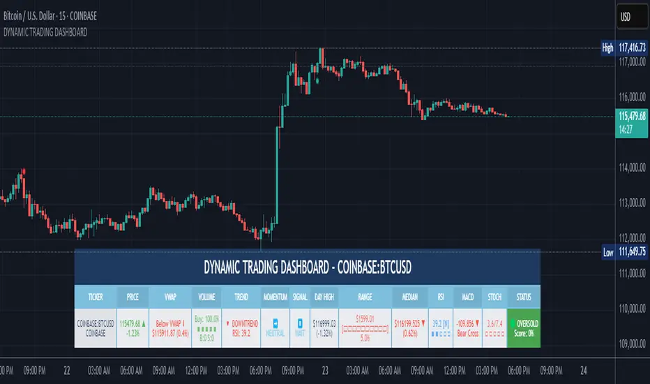
All TimeFrame OscillatorsI have always fighted to understand the market direction because it looks different on different timeframes.
I wanted an indicator where I can see all the different timeframes at once.
This indicator shows already existing oscillators but not only in the current chart's timeframe, but all the most important higer timeframes at once.
I have started with the stoch, then added as many oscillators as I could.
Experimenting with this I have saw that confluence of 4H 1D and 1W Stoch can be very interesting and can highlight higher timeframe take profit areas and sometimes major tops/bottoms.
Also bounces can be interesting when a lower timeframe stoch is bounced or rejected from a higher one.
Oscillators:
Stoch - Stochastic Oscillator
SMI - Stochastic Momentum Index
Rsi - Relative Strength Index
StochRsi - Stochastic RSI
WaveTrend - Vumanchu alias Market Cypher Wave Trend line
CCI - Commodity Channel Index
CCIStoch - Stochastic CCI
Williams Percent Range - Williams %R
Norm. MACD - Normalized Moving Average Convergence Divergence
Norm. MACD Hist - Normalized MACD Histogramm
PVT - Normalized Price Volume Trend
MFI - Money Flow Index
CMF - Chaikin Money Flow
Chande Momentum - Chande Momentum
Volume - Normalized Volume
CandleValue - Vumanchu alias Market Cypher MoneyFlow
BBWP - Bollinger Band Width Percentile
Line Type
Smooth: lines are smoothed, but the actualy not closed values are not shown
Step: Step lines, the actually open timeframes are calculated as they closed at the current values
Plot Oscillator or it's Slope:
its possible to not plot the oscillator but it's slope
Print dots when:
Cross Up/Down oversold/overbougt level - best for most oscillators. for example when Stoch crosses above 20 or below 80
Cross os/ob and the one higher TF is about to cross - when it's crosses beolw 80 and the higher timeframe oscillator is still above ans sloping down
Cross above/below middle line - for example on RSI being above or below 50 can be interesting
Print triangles when:
All Slope Match - all visible timeframe lines are pointing up or down at the same time
All above/belove middle line - all visible lines are above or belove the middle line
All above/belove middle line and slope match - like the previous one and the slope direction is the same
All above/below oversold/overbougt - all lines are above or below os/ ob. this is the default. it can be a very important confluence
Lower TF in order - 5, 15, 30, 60 minute timeframes are in order.
Higher TF in order - 4H 1D 1W in order (like 4H above 1D abd 1D above 1W). can be interesting at RSI
4H-1D in order - 4H 1D in order .
Print triangles
Print all triangles - print all triangles when the condition is met
Print only first triangles - only show when the condition starts to met
Print only last triangles - small triangles when the condition met first, large when last. tis is the default.
Timeframes to show:
You can turn on/off different timeframs to show or not from the list below:
1m 5m 15m 30m 1H 4H D 5D W M
This is for experimenting/ understanding the market direction on multiple timeframes at once.
Don't take it's signals (and any other indicator's) as exact trade signals. use it as confirmation instead.
Any comments, insights, ideas are welcome.

[COG]TMS Crossfire 🔍 TMS Crossfire: Guide to Parameters
📊 Core Parameters
🔸 Stochastic Settings (K, D, Period)
- **What it does**: These control how the first stochastic oscillator works. Think of it as measuring momentum speed.
- **K**: Determines how smooth the main stochastic line is. Lower values (1-3) react quickly, higher values (3-9) are smoother.
- **D**: Controls the smoothness of the signal line. Usually kept equal to or slightly higher than K.
- **Period**: How many candles are used to calculate the stochastic. Standard is 14 days, lower for faster signals.
- **For beginners**: Start with the defaults (K:3, D:3, Period:14) until you understand how they work.
🔸 Second Stochastic (K2, D2, Period2)
- **What it does**: Creates a second, independent stochastic for stronger confirmation.
- **How to use**: Can be set identical to the first one, or with slightly different values for dual confirmation.
- **For beginners**: Start with the same values as the first stochastic, then experiment.
🔸 RSI Length
- **What it does**: Controls the period for the RSI calculation, which measures buying/selling pressure.
- **Lower values** (7-9): More sensitive, good for short-term trading
- **Higher values** (14-21): More stable, better for swing trading
- **For beginners**: The default of 11 is a good balance between speed and reliability.
🔸 Cross Level
- **What it does**: The centerline where crosses generate signals (default is 50).
- **Traditional levels**: Stochastics typically use 20/80, but 50 works well for this combined indicator.
- **For beginners**: Keep at 50 to focus on trend following strategies.
🔸 Source
- **What it does**: Determines which price data is used for calculations.
- **Common options**:
- Close: Most common and reliable
- Open: Less common
- High/Low: Used for specialized indicators
- **For beginners**: Stick with "close" as it's most commonly used and reliable.
🎨 Visual Theme Settings
🔸 Bullish/Bearish Main
- **What it does**: Sets the overall color scheme for bullish (up) and bearish (down) movements.
- **For beginners**: Green for bullish and red for bearish is intuitive, but choose any colors that are easy for you to distinguish.
🔸 Bullish/Bearish Entry
- **What it does**: Colors for the entry signals shown directly on the chart.
- **For beginners**: Use bright, attention-grabbing colors that stand out from your chart background.
🌈 Line Colors
🔸 K1, K2, RSI (Bullish/Bearish)
- **What it does**: Controls the colors of each indicator line based on market direction.
- **For beginners**: Use different colors for each line so you can quickly identify which line is which.
⏱️ HTF (Higher Timeframe) Settings
🔸 HTF Timeframe
- **What it does**: Sets which higher timeframe to use for filtering (e.g., 240 = 4 hour chart).
- **How to choose**: Should be at least 4x your current chart timeframe (e.g., if trading on 15min, use 60min or higher).
- **For beginners**: Start with a timeframe 4x higher than your trading chart.
🔸 Use HTF Filter
- **What it does**: Toggles whether the higher timeframe filter is applied or not.
- **For beginners**: Keep enabled to reduce false signals, especially when learning.
🔸 HTF Confirmation Bars
- **What it does**: How many bars must confirm a trend change on higher timeframe.
- **Higher values**: More reliable but slower to react
- **Lower values**: Faster signals but more false positives
- **For beginners**: Start with 2-3 bars for a good balance.
📈 EMA Settings
🔸 Use EMA Filter
- **What it does**: Toggles price filtering with an Exponential Moving Average.
- **For beginners**: Keep enabled for better trend confirmation.
🔸 EMA Period
- **What it does**: Length of the EMA for filtering (shorter = faster reactions).
- **Common values**:
- 5-13: Short-term trends
- 21-50: Medium-term trends
- 100-200: Long-term trends
- **For beginners**: 5-10 is good for short-term trading, 21 for swing trading.
🔸 EMA Offset
- **What it does**: Shifts the EMA forward or backward on the chart.
- **For beginners**: Start with 0 and adjust only if needed for visual clarity.
🔸 Show EMA on Chart
- **What it does**: Toggles whether the EMA appears on your main price chart.
- **For beginners**: Keep enabled to see how price relates to the EMA.
🔸 EMA Color, Style, Width, Transparency
- **What it does**: Customizes how the EMA line looks on your chart.
- **For beginners**: Choose settings that make the EMA visible but not distracting.
🌊 Trend Filter Settings
🔸 Use EMA Trend Filter
- **What it does**: Enables a multi-EMA system that defines the overall market trend.
- **For beginners**: Keep enabled for stronger trend confirmation.
🔸 Show Trend EMAs
- **What it does**: Toggles visibility of the trend EMAs on your chart.
- **For beginners**: Enable to see how price moves relative to multiple EMAs.
🔸 EMA Line Thickness
- **What it does**: Controls how the thickness of EMA lines is determined.
- **Options**:
- Uniform: All EMAs have the same thickness
- Variable: Each EMA has its own custom thickness
- Hierarchical: Automatically sized based on period (longer periods = thicker)
- **For beginners**: "Hierarchical" is most intuitive as longer-term EMAs appear more dominant.
🔸 EMA Line Style
- **What it does**: Sets the line style (solid, dotted, dashed) for all EMAs.
- **For beginners**: "Solid" is usually clearest unless you have many lines overlapping.
🎭 Trend Filter Colors/Width
🔸 EMA Colors (8, 21, 34, 55)
- **What it does**: Sets the color for each individual trend EMA.
- **For beginners**: Use a logical progression (e.g., shorter EMAs brighter, longer EMAs darker).
🔸 EMA Width Settings
- **What it does**: Controls the thickness of each EMA line.
- **For beginners**: Thicker lines for longer EMAs make them easier to distinguish.
🔔 How These Parameters Work Together
The power of this indicator comes from how these components interact:
1. **Base Oscillator**: The stochastic and RSI components create the main oscillator
2. **HTF Filter**: The higher timeframe filter prevents trading against larger trends
3. **EMA Filter**: The EMA filter confirms signals with price action
4. **Trend System**: The multi-EMA system identifies the overall market environment
Think of it as multiple layers of confirmation, each adding more reliability to your trading signals.
💡 Tips for Beginners
1. **Start with defaults**: Use the default settings first and understand what each element does
2. **One change at a time**: When customizing, change only one parameter at a time
3. **Keep notes**: Write down how each change affects your results
4. **Backtest thoroughly**: Test any changes on historical data before trading real money
5. **Less is more**: Sometimes simpler settings work better than complicated ones
Remember, no indicator is perfect - always combine this with proper risk management and other forms of analysis!
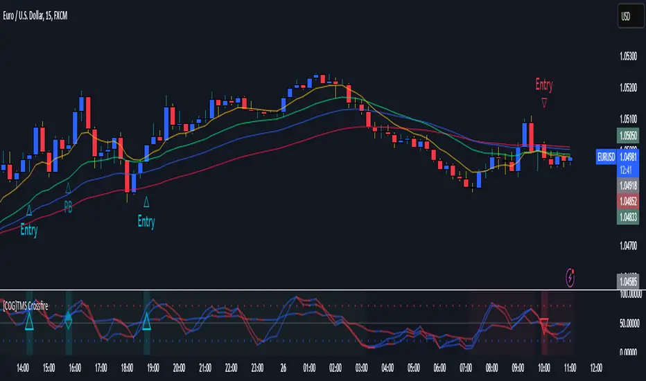
MULTI_Rsi3 - multiple rsi of 4 valuesThis is a MULti RSI with STOCH included which I programmed, it has the option of up to 4 RSI in different values and a STOCH, I hope it serves them, it is very useful when not having so many indicators at the same time.
easy configuration of each RSI, both in value and color, also for the STOCH.
Este es un MULti RSI con STOCH incluido el cual programé, tiene la opción de hasta 4 RSI en diferentes valores y un STOCH, espero les sirve, es muy útil a la hora de no tener tantos indicadores al mismo tiempo.
facil configuración de cada RSI, tanto en valor como en color, igualmente para el STOCH.
