Fisher Transform Trend Navigator [QuantAlgo]🟢 Overview
The Fisher Transform Trend Navigator applies a logarithmic transformation to normalize price data into a Gaussian distribution, then combines this with volatility-adaptive thresholds to create a trend detection system. This mathematical approach helps traders identify high-probability trend changes and reversal points while filtering market noise in the ever-changing volatility conditions.
🟢 How It Works
The indicator's foundation begins with price normalization, where recent price action is scaled to a bounded range between -1 and +1:
highestHigh = ta.highest(priceSource, fisherPeriod)
lowestLow = ta.lowest(priceSource, fisherPeriod)
value1 = highestHigh != lowestLow ? 2 * (priceSource - lowestLow) / (highestHigh - lowestLow) - 1 : 0
value1 := math.max(-0.999, math.min(0.999, value1))
This normalized value then passes through the Fisher Transform calculation, which applies a logarithmic function to convert the data into a Gaussian normal distribution that naturally amplifies price extremes and turning points:
fisherTransform = 0.5 * math.log((1 + value1) / (1 - value1))
smoothedFisher = ta.ema(fisherTransform, fisherSmoothing)
The smoothed Fisher signal is then integrated with an exponential moving average to create a hybrid trend line that balances statistical precision with price-following behavior:
baseTrend = ta.ema(close, basePeriod)
fisherAdjustment = smoothedFisher * fisherSensitivity * close
fisherTrend = baseTrend + fisherAdjustment
To filter out false signals and adapt to market conditions, the system calculates dynamic threshold bands using volatility measurements:
dynamicRange = ta.atr(volatilityPeriod)
threshold = dynamicRange * volatilityMultiplier
upperThreshold = fisherTrend + threshold
lowerThreshold = fisherTrend - threshold
When price momentum pushes through these thresholds, the trend line locks onto the new level and maintains direction until the opposite threshold is breached:
if upperThreshold < trendLine
trendLine := upperThreshold
if lowerThreshold > trendLine
trendLine := lowerThreshold
🟢 Signal Interpretation
Bullish Candles (Green): indicate normalized price distribution favoring bulls with sustained buying momentum = Long/Buy opportunities
Bearish Candles (Red): indicate normalized price distribution favoring bears with sustained selling pressure = Short/Sell opportunities
Upper Band Zone: Area above middle level indicating statistically elevated trend strength with potential overbought conditions approaching mean reversion zones
Lower Band Zone: Area below middle level indicating statistically depressed trend strength with potential oversold conditions approaching mean reversion zones
Built-in Alert System: Automated notifications trigger when bullish or bearish states change, allowing you to act on significant developments without constantly monitoring the charts
Candle Coloring: Optional feature applies trend colors to price bars for visual consistency and clarity
Configuration Presets: Three parameter sets available - Default (balanced settings), Scalping (faster response with higher sensitivity), and Swing Trading (slower response with enhanced smoothing)
Color Customization: Four color schemes including Classic, Aqua, Cosmic, and Custom options for personalized chart aesthetics
Xauusd(w)

Laguerre Filter Trend Navigator [QuantAlgo]🟢 Overview
The Laguerre Filter Trend Navigator employs advanced polynomial filtering mathematics to smooth price data while minimizing lag, creating a responsive yet stable trend-following system. Unlike simple moving averages that apply equal weight to historical data, the Laguerre filter uses recursive calculations with exponentially weighted polynomials to extract meaningful directional signals from noisy market conditions. Combined with dynamic volatility-adjusted boundaries, this creates an adaptive framework for identifying high-probability trend reversals and continuations across all tradable instruments and timeframes.
🟢 How It Works
The indicator leverages Laguerre polynomial filtering, a mathematical technique originally developed for digital signal processing applications. The core mechanism processes price data through four cascaded filter stages (L0, L1, L2, L3), each applying the gamma coefficient to recursively smooth incoming information while preserving phase relationships. This multi-stage architecture eliminates random fluctuations more effectively than traditional moving averages while responding quickly to genuine directional shifts.
The gamma coefficient serves as the primary smoothing control, determining how aggressively the filter dampens noise versus tracking price movements. Lower gamma values reduce smoothing and increase filter responsiveness, while higher values prioritize stability over reaction speed. Each filter stage compounds this effect, creating progressively smoother output that converges toward true underlying trend direction.
Surrounding the filtered price line, the algorithm constructs adaptive boundaries using dynamic volatility regime measurements. These calculations quantify current market turbulence independently of direction, expanding during active trading periods and contracting during quiet phases. By multiplying this volatility assessment by a user-defined scaling factor, the system creates self-adjusting bands that automatically conform to changing market conditions without manual intervention.
The trend-following engine monitors price position relative to these volatility-adjusted boundaries. When the upper band falls below the current trend line, the system shifts downward to track bearish momentum. Conversely, when the lower band rises above the trend line, it elevates to follow bullish movement. These crossover events trigger color transitions between bullish (green) and bearish (red) states, providing clear visual confirmation of directional changes validated by volatility-normalized thresholds.
🟢 How to Use
Green/Bullish Trend Line: Laguerre filter positioned in upward trajectory, indicating momentum-confirmed conditions favorable for establishing or maintaining long positions (buy)
Red/Bearish Trend Line: Laguerre filter trending downward, signaling regime-validated environment suitable for initiating or holding short positions (sell)
Rising Green Line: Accelerating bullish filter with expanding separation from price lows, demonstrating strengthening upward momentum and increasing confidence in trend persistence with optimal long entry timing
Declining Red Line: Steepening bearish filter creating growing distance from price highs, revealing intensifying downside pressure and enhanced probability of continued decline with favorable short positioning opportunities
Flattening Trends: Horizontal or oscillating filter movement regardless of color suggests directional uncertainty where price action contradicts filter positioning, potentially indicating consolidation phases or impending volatility expansion requiring cautious trade management
🟢 Pro Tips for Trading and Investing
→ Preset Selection Framework: Match presets to your trading style - Scalping preset employs aggressive gamma (0.4) with tight volatility bands (1.0x) for rapid signal generation on sub-15-minute charts, Day Trading preset balances responsiveness and stability for hourly timeframes, while Swing Trading preset maximizes smoothing (0.8 gamma) with wide bands (2.5x) to filter intraday noise on daily and weekly charts.
→ Gamma Coefficient Calibration: Adjust gamma based on market personality - reduce values (0.3-0.5) for highly liquid, fast-moving assets like major currency pairs and tech stocks where quick filter adaptation prevents lag-induced losses, increase values (0.7-0.9) for slower instruments or trending markets where excessive sensitivity generates false reversals and whipsaw trades.
→ Volatility Period Optimization: Tailor the volatility measurement window to information cycles. Deploy shorter lookback periods (7-10) for instruments with rapid regime changes like individual equities during earnings seasons, standard periods (14-20) for balanced assessment across general market conditions, and extended periods (21-30) for commodities and indices exhibiting persistent volatility characteristics.
→ Band Width Multiplier Adaptation: Scale boundary distance to current market phase. Contract multipliers (1.0-1.5) during range-bound consolidations to capture early breakout signals as soon as genuine momentum emerges, expand multipliers (2.0-3.0) during trending markets or high-volatility events to avoid premature exits caused by normal retracement activity rather than authentic reversals.
→ Multi-Timeframe Filter Alignment: Implement the indicator across multiple timeframes, using higher intervals (4H/Daily) to identify primary trend direction via filter slope and lower intervals (15min/1H) for precision entry timing when filter colors align, ensuring trades flow with dominant momentum while optimizing execution at favorable price levels.
→ Alert-Driven Systematic Execution: Configure trend change alerts to capture every filter-validated directional shift from bullish to bearish conditions or vice versa, enabling consistent signal response without continuous chart monitoring and eliminating emotional decision-making during critical transition moments.

Bayesian Trend Navigator [QuantAlgo]🟢 Overview
The Bayesian Trend Navigator uses Bayesian statistics to continuously update trend probabilities by combining long-term expectations (prior beliefs) and short-term observations (likelihood evidence), rather than relying solely on recent price data like many conventional indicators. This mathematical framework produces robust directional signals that naturally balance responsiveness with stability, making it suitable for traders and investors seeking statistically-grounded trend identification across diverse market environments and asset types.
🟢 How It Works
The indicator operates on Bayesian inference principles, a statistical method for updating beliefs when new evidence emerges. The system begins by establishing a prior belief - a long-term trend expectation calculated from historical price behavior. This represents the "baseline hypothesis" about market direction before considering recent developments.
Simultaneously, the algorithm collects recent market evidence through short-term trend analysis, representing the likelihood component. This captures what current price action suggests about directional momentum independent of historical context.
The core Bayesian engine then combines these elements using conjugate normal distributions and precision weighting. It calculates prior precision (inverse variance) and likelihood precision, combining them to determine a posterior precision. The resulting posterior mean represents the mathematically optimal trend estimate given both historical patterns and current reality. This posterior calculation includes intervals derived from the posterior variance, providing probabilistic confidence bounds around the trend estimate.
Finally, volatility-based standard deviation bands create adaptive boundaries around the Bayesian estimate. The trend line adjusts within these constraints, generating color transitions between bullish (green) and bearish (red) states when the posterior calculation crosses these probabilistic thresholds.
🟢 How to Use
Green/Bullish Trend Line: Posterior probability favoring upward momentum, indicating statistically favorable conditions for long positions (buy)
Red/Bearish Trend Line: Posterior probability favoring downward momentum, signaling mathematically supported timing for short positions (sell)
Rising Green Line: Strengthening bullish posterior as new evidence reinforces upward beliefs, showing increasing probabilistic confidence in trend continuation with favorable long entry conditions
Declining Red Line: Intensifying bearish posterior with accumulating downside evidence, indicating growing statistical certainty in downtrend persistence and optimal short positioning opportunities
Flattening Trends: Diminishing posterior confidence regardless of color suggests equilibrium between prior beliefs and contradictory evidence, potentially signaling consolidation or insufficient statistical clarity for high-conviction trades
🟢 Pro Tips for Trading and Investing
→ Preset Configuration Strategy: Deploy presets based on your trading horizon - Scalping preset maximizes evidence weight (0.8) for rapid Bayesian updates on 1-15 minute charts, Default preset balances prior and likelihood for general applications, while Swing Trading preset equalizes weights (0.5/0.5) for stable inference on hourly and daily timeframes.
→ Prior Weight Adjustment: Calibrate prior weight according to market regime - increase values (0.5-0.7) in stable trending markets where historical patterns remain predictive, decrease values (0.2-0.3) during regime changes or news-driven volatility when recent evidence should dominate the posterior calculation.
→ Evidence Period Tuning: Modify the evidence period based on information flow velocity. Use shorter periods (5-8 bars) for assets with continuous price discovery like cryptocurrencies, medium periods (10-15) for liquid stocks, and longer periods (15-20) for slower-moving markets to ensure adequate likelihood sample size.
→ Likelihood Weight Optimization: Adjust likelihood weight inversely to market noise levels. Higher values (0.7-0.8) work well in clean trending conditions where recent data is reliable, while lower values (0.4-0.6) help during choppy periods by maintaining stronger reliance on established prior beliefs.
→ Multi-Timeframe Bayesian Confluence: Apply the indicator across multiple timeframes, using higher timeframes (Daily/Weekly) to establish prior belief direction and lower timeframes (Hourly/15-minute) for likelihood-driven entry timing, ensuring posterior probabilities align across temporal scales for maximum statistical confidence.
→ Standard Deviation Multiplier Management: Adapt the multiplier to match current uncertainty levels. Use tighter multipliers (1.0-1.5) during low-volatility consolidations to capture early trend emergence, and wider multipliers (2.0-2.5) during high-volatility events to avoid premature signals caused by statistical noise rather than genuine posterior shifts.
→ Variance-Based Position Sizing: Monitor the implicit posterior variance through trend line stability - smooth consistent movements indicate low uncertainty warranting larger positions, while erratic fluctuations suggest high statistical uncertainty calling for reduced exposure until clearer probabilistic convergence emerges.
→ Alert-Based Probabilistic Execution: Utilize trend change alerts to capture every statistically significant posterior shift from bullish to bearish states or vice versa without constantly monitoring the charts.

MACD Forecast [Titans_Invest]MACD Forecast — The Future of MACD in Trading
The MACD has always been one of the most powerful tools in technical analysis.
But what if you could see where it’s going, instead of just reacting to what has already happened?
Introducing MACD Forecast — the natural evolution of the MACD Full , now taken to the next level. It’s the world’s first MACD designed not only to analyze the present but also to predict the future behavior of momentum.
By combining the classic MACD structure with projections powered by Linear Regression, this indicator gives traders an anticipatory, predictive view, redefining what’s possible in technical analysis.
Forget lagging indicators.
This is the smartest, most advanced, and most accurate MACD ever created.
🍟 WHY MACD FORECAST IS REVOLUTIONARY
Unlike the traditional MACD, which only reflects current and past price dynamics, the MACD Forecast uses regression-based projection models to anticipate where the MACD line, signal line, and histogram are heading.
This means traders can:
• See MACD crossovers before they happen.
• Spot trend reversals earlier than most.
• Gain an unprecedented timing advantage in both discretionary and automated trading.
In other words: this indicator lets you trade ahead of time.
🔮 FORECAST ENGINE — POWERED BY LINEAR REGRESSION
At its core, the MACD Forecast integrates Linear Regression (ta.linreg) to project the MACD’s future behavior with exceptional accuracy.
Projection Modes:
• Flat Projection: Assumes trend continuity at the current level.
• LinReg Projection: Applies linear regression across N periods to mathematically forecast momentum shifts.
This dual system offers both a conservative and adaptive view of market direction.
📐 ACCURACY WITH FULL CUSTOMIZATION
Just like the MACD Full, this new version comes with 20 customizable buy-entry conditions and 20 sell-entry conditions — now enhanced with forecast-based rules that anticipate crossovers and trend reversals.
You’re not just reacting — you’re strategizing ahead of time.
⯁ HOW TO USE MACD FORECAST❓
The MACD Forecast is built on the same foundation as the classic MACD, but with predictive capabilities.
Step 1 — Spot Predicted Crossovers:
Watch for forecasted bullish or bearish crossovers. These signals anticipate when the MACD line will cross the signal line in the future, letting you prepare trades before the move.
Step 2 — Confirm with Histogram Projection:
Use the projected histogram to validate momentum direction. A rising histogram signals strengthening bullish momentum, while a falling projection points to weakening or bearish conditions.
Step 3 — Combine with Multi-Timeframe Analysis:
Use forecasts across multiple timeframes to confirm signal strength (e.g., a 1h forecast aligned with a 4h forecast).
Step 4 — Set Entry Conditions & Automation:
Customize your buy/sell rules with the 20 forecast-based conditions and enable automation for bots or alerts.
Step 5 — Trade Ahead of the Market:
By preparing for future momentum shifts instead of reacting to the past, you’ll always stay one step ahead of lagging traders.
🤖 BUILT FOR AUTOMATION AND BOTS 🤖
Whether for manual trading, quantitative strategies, or advanced algorithms, the MACD Forecast was designed to integrate seamlessly with automated systems.
With predictive logic at its core, your strategies can finally react to what’s coming, not just what already happened.
🥇 WHY THIS INDICATOR IS UNIQUE 🥇
• World’s first MACD with Linear Regression Forecasting
• Predictive Crossovers (before they appear on the chart)
• Maximum flexibility with Long & Short combinations — 20+ fully configurable conditions for tailor-made strategies
• Fully automatable for quantitative systems and advanced bots
This isn’t just an update.
It’s the final evolution of the MACD.
______________________________________________________
🔹 CONDITIONS TO BUY 📈
______________________________________________________
• Signal Validity: The signal will remain valid for X bars .
• Signal Sequence: Configurable as AND or OR .
🔹 MACD > Signal Smoothing
🔹 MACD < Signal Smoothing
🔹 Histogram > 0
🔹 Histogram < 0
🔹 Histogram Positive
🔹 Histogram Negative
🔹 MACD > 0
🔹 MACD < 0
🔹 Signal > 0
🔹 Signal < 0
🔹 MACD > Histogram
🔹 MACD < Histogram
🔹 Signal > Histogram
🔹 Signal < Histogram
🔹 MACD (Crossover) Signal
🔹 MACD (Crossunder) Signal
🔹 MACD (Crossover) 0
🔹 MACD (Crossunder) 0
🔹 Signal (Crossover) 0
🔹 Signal (Crossunder) 0
🔮 MACD (Crossover) Signal Forecast
🔮 MACD (Crossunder) Signal Forecast
______________________________________________________
______________________________________________________
🔸 CONDITIONS TO SELL 📉
______________________________________________________
• Signal Validity: The signal will remain valid for X bars .
• Signal Sequence: Configurable as AND or OR .
🔸 MACD > Signal Smoothing
🔸 MACD < Signal Smoothing
🔸 Histogram > 0
🔸 Histogram < 0
🔸 Histogram Positive
🔸 Histogram Negative
🔸 MACD > 0
🔸 MACD < 0
🔸 Signal > 0
🔸 Signal < 0
🔸 MACD > Histogram
🔸 MACD < Histogram
🔸 Signal > Histogram
🔸 Signal < Histogram
🔸 MACD (Crossover) Signal
🔸 MACD (Crossunder) Signal
🔸 MACD (Crossover) 0
🔸 MACD (Crossunder) 0
🔸 Signal (Crossover) 0
🔸 Signal (Crossunder) 0
🔮 MACD (Crossover) Signal Forecast
🔮 MACD (Crossunder) Signal Forecast
______________________________________________________
______________________________________________________
🔮 Linear Regression Function 🔮
______________________________________________________
• Our indicator includes MACD forecasts powered by linear regression.
Forecast Types:
• Flat: Assumes prices will stay the same.
• Linreg: Makes a 'Linear Regression' forecast for n periods.
Technical Information:
• Function: ta.linreg()
Parameters:
• source: Source price series.
• length: Number of bars (period).
• offset : Offset.
• return: Linear regression curve.
______________________________________________________
______________________________________________________
⯁ UNIQUE FEATURES
______________________________________________________
Linear Regression: (Forecast)
Signal Validity: The signal will remain valid for X bars
Signal Sequence: Configurable as AND/OR
Table of Conditions: BUY/SELL
Conditions Label: BUY/SELL
Plot Labels in the graph above: BUY/SELL
Automate & Monitor Signals/Alerts: BUY/SELL
Linear Regression (Forecast)
Signal Validity: The signal will remain valid for X bars
Signal Sequence: Configurable as AND/OR
Table of Conditions: BUY/SELL
Conditions Label: BUY/SELL
Plot Labels in the graph above: BUY/SELL
Automate & Monitor Signals/Alerts: BUY/SELL
______________________________________________________
📜 SCRIPT : MACD Forecast
🎴 Art by : @Titans_Invest & @DiFlip
👨💻 Dev by : @Titans_Invest & @DiFlip
🎑 Titans Invest — The Wizards Without Gloves 🧤
✨ Enjoy!
______________________________________________________
o Mission 🗺
• Inspire Traders to manifest Magic in the Market.
o Vision 𐓏
• To elevate collective Energy 𐓷𐓏
🎗️ In memory of João Guilherme — your light will live on forever.

Maple Algorithm_GOLDMaple Algorithm – AI-Powered Gold Indicator
Maple Algorithm is an AI-inspired indicator designed specifically around the price behavior of Gold (XAUUSD).
It automatically calculates and plots take-profit (TP) and stop-loss (SL) levels based on dynamic market conditions, allowing traders to capture precise entries and exits.
✨ Key Features
AI-driven adaptive model trained on Gold’s market structure
Auto-generated TP/SL zones for precision trading
Compatible with your own strategies — scale from 1:2 RRR up to even higher setups
Optimized for scalping and short-term momentum bursts
⚠️ Disclaimer:
This indicator is for educational and research purposes only. It does not guarantee future results. Always test thoroughly before applying to live trading.
VOLUME Full [Titans_Invest]VOLUME Full
Designed for traders who want to take volume analysis to the next level.
This version delivers deeper insight into volume activity, integrating multiple customizable filters to highlight key buying and selling pressure. It's a comprehensive solution for volume-based decision-making.
⯁ WHAT IS THE VOLUME❓
The Volume indicator is a fundamental technical analysis tool that measures the number of shares or contracts traded in a security or market during a given period. It helps traders and investors understand the strength or weakness of a price movement, confirm trends, and predict potential reversals. Volume is typically displayed as a histogram below a price chart, with each bar representing the volume traded during a specific time interval.
⯁ HOW TO USE THE VOLUME❓
The Volume indicator can be used in several ways to enhance trading decisions:
• Trend Confirmation: High volume during a price move confirms the strength of that trend, while low volume can indicate a weak or unsustainable trend.
• Breakouts: A price breakout from a pattern or range accompanied by high volume is more likely to be valid and sustainable.
• Divergence: When the price moves in one direction and volume moves in the opposite direction, it can signal a potential reversal.
• Overbought/Oversold Conditions: Extreme volume levels can sometimes indicate that an asset is overbought or oversold, though this is less straightforward than with oscillators like the RSI.
⯁ ENTRY CONDITIONS
The conditions below are fully flexible and allow for complete customization of the signal.
______________________________________________________
🔹 CONDITIONS TO BUY 📈
______________________________________________________
▪︎ Signal Validity: The signal will remain valid for X bars .
▪︎ Signal Sequence: Configurable as AND or OR .
🔹 volume Positive
🔹 volume Negative
🔹 volume > volume
🔹 volume < volume
🔹 volume > volume_MA
🔹 volume > volume_MA * Trigger Signal (close > open)
🔹 volume > volume_MA * Trigger Signal (Keep State P)
🔹 volume > volume_MA * Trigger Signal (close < open)
🔹 volume > volume_MA * Trigger Signal (Keep State N)
______________________________________________________
______________________________________________________
🔸 CONDITIONS TO SELL 📉
______________________________________________________
▪︎ Signal Validity: The signal will remain valid for X bars .
▪︎ Signal Sequence: Configurable as AND or OR .
🔸 volume Positive
🔸 volume Negative
🔸 volume > volume
🔸 volume < volume
🔸 volume > volume_MA
🔸 volume > volume_MA * Trigger Signal (close > open)
🔸 volume > volume_MA * Trigger Signal (Keep State P)
🔸 volume > volume_MA * Trigger Signal (close < open)
🔸 volume > volume_MA * Trigger Signal (Keep State N)
______________________________________________________
______________________________________________________
🤖 AUTOMATION 🤖
• You can automate the BUY and SELL signals of this indicator.
______________________________________________________
______________________________________________________
⯁ UNIQUE FEATURES
______________________________________________________
Signal Validity: The signal will remain valid for X bars
Signal Sequence: Configurable as AND/OR
Condition Table: BUY/SELL
Condition Labels: BUY/SELL
Plot Labels in the Graph Above: BUY/SELL
Displays Positive & Negative Volume.
Automate and Monitor Signals/Alerts: BUY/SELL
Signal Validity: The signal will remain valid for X bars
Signal Sequence: Configurable as AND/OR
Table of Conditions: BUY/SELL
Conditions Label: BUY/SELL
Plot Labels in the graph above: BUY/SELL
Displays Positive & Negative Volume.
Automate & Monitor Signals/Alerts: BUY/SELL
______________________________________________________
📜 SCRIPT : VOLUME Full
🎴 Art by : @Titans_Invest & @DiFlip
👨💻 Dev by : @Titans_Invest & @DiFlip
🎑 Titans Invest — The Wizards Without Gloves 🧤
✨ Enjoy!
______________________________________________________
o Mission 🗺
• Inspire Traders to manifest Magic in the Market.
o Vision 𐓏
• To elevate collective Energy 𐓷𐓏

Apex Edge Sentinel - Stop Loss HUDApex Edge – ATR Sentinel Stop Loss HUD
The Apex Edge – ATR Sentinel is a complete stop-loss intelligence system built as a clean, always-on HUD.
It delivers institutional-level risk guidance by calculating and displaying live ATR-based stop levels for both long and short trades at multiple risk tolerances.
Forget cluttered charts and repainting lines — Sentinel gives you a clear stop-loss reference panel that updates dynamically with every bar.
✅ Features
• Triple ATR Multipliers
User-defined (e.g. x1.5 / x2.0 / x2.5). Compare tight, medium, and wide stops instantly.
• Dual-Side SL Levels
Both Long and Short safe stop prices displayed side by side. No more guessing trend
bias.
• ATR Transparency
HUD shows ATR(length) so you always know the calculation basis. Default = 14, adjustable
to your style.
• ATR Regime Meter
Detects volatility conditions (LOW / NORMAL / HIGH) by comparing ATR to its SMA. Helps
you avoid over-tight stops in high-volatility markets.
• Tick-Aware Rounding
Stop levels auto-rounded to the instrument’s tick size (Gold = 0.10, FX = 0.0001, indices =
whole points).
Custom HUD Design
• Location: Top/Bottom, Left/Right
• Sizes: Compact / Medium / Large (desktop or mobile)
• Opacity control (25% default Apex styling)
How to Use
1. Load Sentinel on your chart.
2. Check the HUD:
• ATR(14): 2.6 → base volatility measure.
• x1.5 / x2.0 / x2.5 → instant SL levels for both long & short trades.
3. Before entering a trade → decide which multiplier matches your style (tight scalper vs wider swing).
4. Manually place your SL at the level displayed in the HUD.
Sentinel works as both:
• A pre-trade check (is ATR stop too wide for my RR?).
• A live risk compass (updated stop levels every bar).
Why Apex Sentinel?
Most ATR stop indicators clutter charts with lagging lines or repainting trails. Sentinel strips it back to what matters:
• The numbers.
• The risk levels.
• The context.
It’s a pure stop-loss HUD, designed for serious traders who want clarity, discipline, and instant reference points across any market or timeframe.
Notes
• This is a HUD-only system (no automatic SL line). Traders manually apply the SL level
shown in the panel.
• Defaults: ATR(14), multipliers 1.5 / 2.0 / 2.5. Adjust to your trading style.
• Best used on intraday pairs like XAUUSD, EURUSD, indices, but works universally.
Apex Edge Philosophy: Clean. Smart. Institutional.
No clutter. No gimmicks. Just precision tools for modern markets.
Bollinger Adaptive Trend Navigator [QuantAlgo]🟢 Overview
The Bollinger Adaptive Trend Navigator synthesizes volatility channel analysis with variable smoothing mechanics to generate trend identification signals. It uses price positioning within Bollinger Band structures to modify moving average responsiveness, while incorporating ATR calculations to establish trend line boundaries that constrain movement during volatile periods. The adaptive nature makes this indicator particularly valuable for traders and investors working across various asset classes including stocks, forex, commodities, and cryptocurrencies, with effectiveness spanning multiple timeframes from intraday scalping to longer-term position analysis.
🟢 How It Works
The core mechanism calculates price position within Bollinger Bands and uses this positioning to create an adaptive smoothing factor:
bbPosition = bbUpper != bbLower ? (source - bbLower) / (bbUpper - bbLower) : 0.5
adaptiveFactor = (bbPosition - 0.5) * 2 * adaptiveMultiplier * bandWidthRatio
alpha = math.max(0.01, math.min(0.5, 2.0 / (bbPeriod + 1) * (1 + math.abs(adaptiveFactor))))
This adaptive coefficient drives an exponential moving average that responds more aggressively when price approaches Bollinger Band extremes:
var float adaptiveTrend = source
adaptiveTrend := alpha * source + (1 - alpha) * nz(adaptiveTrend , source)
finalTrend = 0.7 * adaptiveTrend + 0.3 * smoothedCenter
ATR-based volatility boundaries constrain the final trend line to prevent excessive movement during volatile periods:
volatility = ta.atr(volatilityPeriod)
upperBound = bollingerTrendValue + (volatility * volatilityMultiplier)
lowerBound = bollingerTrendValue - (volatility * volatilityMultiplier)
The trend line direction determines bullish or bearish states through simple slope comparison, with the final output displaying color-coded signals based on the synthesis of Bollinger positioning, adaptive smoothing, and volatility constraints (green = long/buy, red = short/sell).
🟢 Signal Interpretation
Rising Trend Line (Green): Indicates upward direction based on Bollinger positioning and adaptive smoothing = Potential long/buy opportunity
Falling Trend Line (Red): Indicates downward direction based on Bollinger positioning and adaptive smoothing = Potential short/sell opportunity
Built-in Alert System: Automated notifications trigger when bullish or bearish states change, allowing you to act on significant development without constantly monitoring the charts
Candle Coloring: Optional feature applies trend colors to price bars for visual consistency
Configuration Presets: Three parameter sets available - Default (standard settings), Scalping (faster response), and Swing Trading (slower response)
Sine Weighted Trend Navigator [QuantAlgo]🟢 Overview
The Sine Weighted Trend Navigator utilizes trigonometric mathematics to create a trend-following system that adapts to various market volatility. Unlike traditional moving averages that apply uniform weights, this indicator employs sine wave calculations to distribute weights across historical price data, creating a more responsive yet smooth trend measurement. Combined with volatility-adjusted boundaries, it produces actionable directional signals for traders and investors across various market conditions and asset classes.
🟢 How It Works
At its core, the indicator applies sine wave mathematics to weight historical prices. The system generates angular values across the lookback period and transforms them through sine calculations, creating a weight distribution pattern that naturally emphasizes recent price action while preserving smoothness. The phase shift feature allows rotation of this weighting pattern, enabling adjustment of the indicator's responsiveness to different market conditions.
Surrounding this sine-weighted calculation, the system establishes volatility-responsive boundaries through market volatility analysis. These boundaries expand and contract based on current market conditions, creating a dynamic framework that helps distinguish meaningful trend movements from random price fluctuations.
The trend determination logic compares the sine-weighted value against these adaptive boundaries. When the weighted value exceeds the upper boundary, it signals upward momentum. When it drops below the lower boundary, it indicates downward pressure. This comparison drives the color transitions of the main trend line, shifting between bullish (green) and bearish (red) states to provide clear directional guidance on price charts.
🟢 How to Use
Green/Bullish Trend Line: Rising momentum indicating optimal conditions for long positions (buy)
Red/Bearish Trend Line: Declining momentum signaling favorable timing for short positions (sell)
Steepening Green Line: Accelerating bullish momentum with increasing sine-weighted values indicating strengthening upward pressure and high-probability trend continuation
Steepening Red Line: Intensifying bearish momentum with declining sine-weighted calculations suggesting persistent downward pressure and optimal shorting opportunities
Flattening Trend Lines: Gradual reduction in directional momentum regardless of color may indicate approaching consolidation or trend exhaustion requiring position management review
🟢 Pro Tips for Trading and Investing
→ Preset Strategy Selection: Utilize the built-in presets strategically - Scalping preset for ultra-responsive 1-15 minute charts, Default preset for balanced general trading, and Swing Trading preset for 1-4 hour charts and multi-day positions.
→ Phase Shift Optimization: Fine-tune the phase shift parameter based on market bias - use positive values (0.1-0.5) in trending bull markets to enhance uptrend sensitivity, negative values (-0.1 to -0.5) in bear markets for improved downtrend detection, and zero for balanced neutral market conditions.
→ Multiplier Calibration: Adjust the multiplier according to market volatility and trading style. Use lower values (0.5-1.0) for tight, responsive signals in stable markets, higher values (2.0-3.0) during earnings seasons or high-volatility periods to filter noise and reduce whipsaws.
→ Sine Period Adaptation: Customize the sine weighted period based on your trading timeframe and market conditions. Use 5-14 for day trading to capture short-term momentum shifts, 14-25 for swing trading to balance responsiveness with reliability, and 25-50 for position trading to maintain long-term trend clarity.
→ Multi-Timeframe Sine Validation: Apply the indicator across multiple timeframes simultaneously, using higher timeframes (4H/Daily) for overall trend bias and lower timeframes (15m/1H) for entry timing, ensuring sine-weighted calculations align across different time horizons.
→ Alert-Driven Systematic Execution: Leverage the built-in trend change alerts to eliminate emotional decision-making and capture every mathematically-confirmed trend transition, particularly valuable for traders managing multiple instruments or those unable to monitor charts continuously.
→ Risk Management: Increase position sizes during strong directional sine-weighted momentum while reducing exposure during frequent color changes that indicate mathematical uncertainty or ranging market conditions lacking clear directional bias.
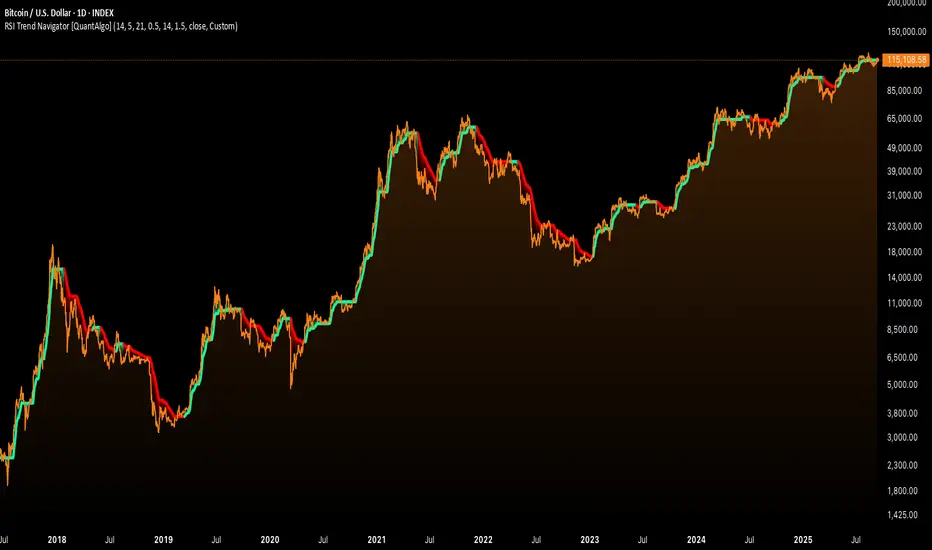
RSI Trend Navigator [QuantAlgo]🟢 Overview
The RSI Trend Navigator integrates RSI momentum calculations with adaptive exponential moving averages and ATR-based volatility bands to generate trend-following signals. The indicator applies variable smoothing coefficients based on RSI readings and incorporates normalized momentum adjustments to position a trend line that responds to both price action and underlying momentum conditions.
🟢 How It Works
The indicator begins by calculating and smoothing the RSI to reduce short-term fluctuations while preserving momentum information:
rsiValue = ta.rsi(source, rsiPeriod)
smoothedRSI = ta.ema(rsiValue, rsiSmoothing)
normalizedRSI = (smoothedRSI - 50) / 50
It then creates an adaptive smoothing coefficient that varies based on RSI positioning relative to the midpoint:
adaptiveAlpha = smoothedRSI > 50 ? 2.0 / (trendPeriod * 0.5 + 1) : 2.0 / (trendPeriod * 1.5 + 1)
This coefficient drives an adaptive trend calculation that responds more quickly when RSI indicates bullish momentum and more slowly during bearish conditions:
var float adaptiveTrend = source
adaptiveTrend := adaptiveAlpha * source + (1 - adaptiveAlpha) * nz(adaptiveTrend , source)
The normalized RSI values are converted into price-based adjustments using ATR for volatility scaling:
rsiAdjustment = normalizedRSI * ta.atr(14) * sensitivity
rsiTrendValue = adaptiveTrend + rsiAdjustment
ATR-based bands are constructed around this RSI-adjusted trend value to create dynamic boundaries that constrain trend line positioning:
atr = ta.atr(atrPeriod)
deviation = atr * atrMultiplier
upperBound = rsiTrendValue + deviation
lowerBound = rsiTrendValue - deviation
The trend line positioning uses these band constraints to determine its final value:
if upperBound < trendLine
trendLine := upperBound
if lowerBound > trendLine
trendLine := lowerBound
Signal generation occurs through directional comparison of the trend line against its previous value to establish bullish and bearish states:
trendUp = trendLine > trendLine
trendDown = trendLine < trendLine
if trendUp
isBullish := true
isBearish := false
else if trendDown
isBullish := false
isBearish := true
The final output colors the trend line green during bullish states and red during bearish states, creating visual buy/long and sell/short opportunity signals based on the combined RSI momentum and volatility-adjusted trend positioning.
🟢 Signal Interpretation
Rising Trend Line (Green): Indicates upward momentum where RSI influence and adaptive smoothing favor continued price advancement = Potential buy/long positions
Declining Trend Line (Red): Indicates downward momentum where RSI influence and adaptive smoothing favor continued price decline = Potential sell/short positions
Flattening Trend Lines: Occur when momentum weakens and the trend line slope approaches neutral, suggesting potential consolidation before the next move
Built-in Alert System: Automated notifications trigger when bullish or bearish states change, sending "RSI Trend Bullish Signal" or "RSI Trend Bearish Signal" messages for timely entry/exit
Color Bar Candles Option: Optional candle coloring feature that applies the same green/red trend colors to price bars, providing additional visual confirmation of the current trend direction
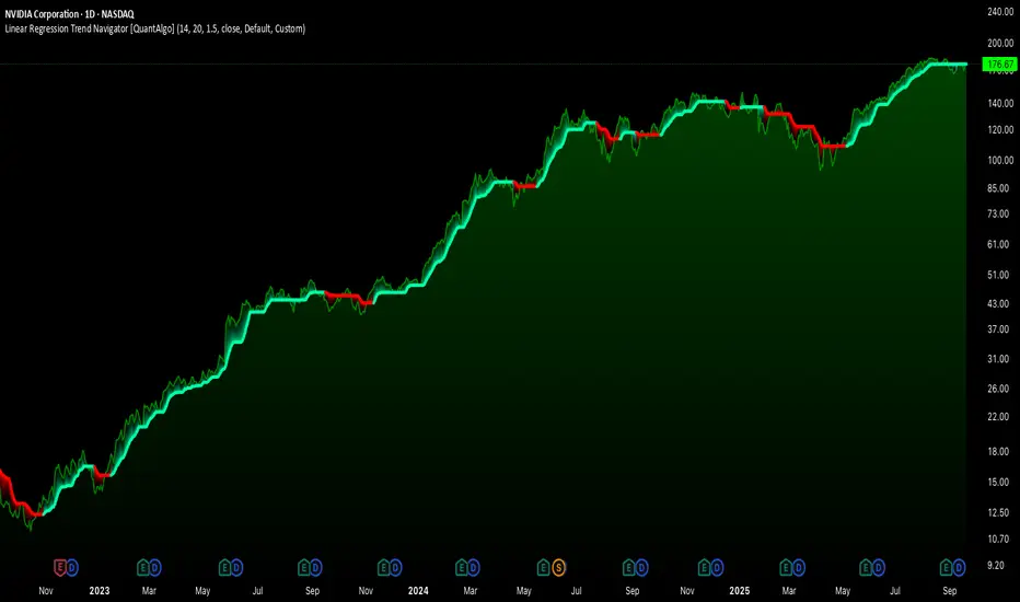
Linear Regression Trend Navigator [QuantAlgo]🟢 Overview
The Linear Regression Trend Navigator is a trend-following indicator that combines statistical regression analysis with adaptive volatility bands to identify and track dominant market trends. It employs linear regression mathematics to establish the underlying trend direction, while dynamically adjusting trend boundaries based on standard deviation calculations to filter market noise and maintain trend continuity. The result is a straightforward visual system where green indicates bullish conditions favoring buy/long positions, and red signals bearish conditions supporting sell/short trades.
🟢 How It Works
The indicator operates through a three-phase computational process that transforms raw price data into adaptive trend signals. In the first phase, it calculates a linear regression line over the specified period, establishing the mathematical best-fit line through recent price action to determine the underlying directional bias. This regression line serves as the foundation for trend analysis by smoothing out short-term price variations while preserving the essential directional characteristics.
The second phase constructs dynamic volatility boundaries by calculating the standard deviation of price movements over the defined period and applying a user-adjustable multiplier. These upper and lower bounds create a volatility-adjusted channel around the regression line, with wider bands during volatile periods and tighter bands during stable conditions. This adaptive boundary system operates entirely behind the scenes, ensuring the trend signal remains relevant across different market volatility regimes without cluttering the visual display.
In the final phase, the system generates a simple trend line that dynamically positions itself within the volatility boundaries. When price action pushes the regression line above the upper bound, the trend line adjusts to the upper boundary level. Conversely, when the regression line falls below the lower bound, the trend line moves to the lower boundary. The result is a single colored line that transitions between green (rising trend line = buy/long) and red (declining trend line = sell/short).
🟢 How to Use
Green Trend Line: Upward momentum indicating favorable conditions for long positions, buy signals, and bullish strategies
Red Trend Line: Downward momentum signaling optimal timing for short positions, sell signals, and bearish approaches
Rising Green Line: Accelerating bullish momentum with steepening angles indicating strengthening upward pressure and potential for trend continuation
Declining Red Line: Intensifying bearish momentum with increasing negative slopes suggesting persistent downward pressure and shorting opportunities
Flattening Trend Lines: Gradual reduction in slope regardless of color may indicate approaching consolidation or momentum exhaustion requiring position review
🟢 Pro Tips for Trading and Investing
→ Entry/Exit Timing: Trade exclusively on band color transitions rather than price patterns, as each color change represents a statistically-confirmed shift that has passed through volatility filtering, providing higher probability setups than traditional technical analysis.
→ Parameter Optimization for Asset Classes: Customize the linear regression period based on your trading style. For example, use 5-10 bars for day trading to capture short-term statistical shifts, 14-20 for swing trading to balance responsiveness with stability, and 25-50 for position trading to filter out medium-term noise.
→ Volatility Calibration Strategy: Adjust the standard deviation multiplier according to market volatility. For instance, increase to 2.0+ during high-volatility periods like earnings or news events to reduce false signals, decrease to 1.0-1.5 during stable market conditions to maintain sensitivity to genuine trends.
→ Cross-Timeframe Statistical Validation: Apply the indicator across multiple timeframes simultaneously, using higher timeframes for directional bias and lower timeframes for entry timing.
→ Alert-Based Systematic Trading: Use built-in alerts to eliminate discretionary decision-making and ensure you capture every statistically-significant trend change, particularly effective for traders who cannot monitor charts continuously.
→ Risk Allocation Based on Signal Strength: Increase position sizes during periods of strong directional movement while reducing exposure during frequent band color changes that indicate statistical uncertainty or ranging conditions.
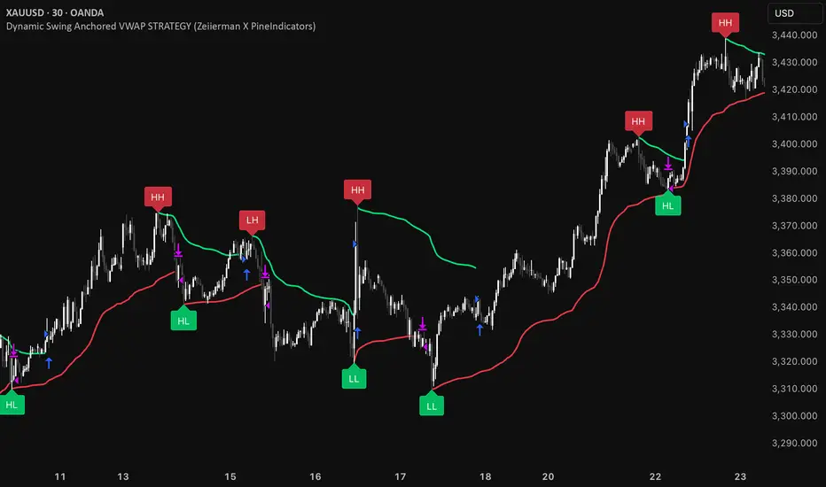
Dynamic Swing Anchored VWAP STRAT (Zeiierman/PineIndicators)Dynamic Swing Anchored VWAP STRATEGY — Zeiierman × PineIndicators (Pine Script v6)
A pivot-to-pivot Anchored VWAP strategy that adapts to volatility, enters long on bullish structure, and closes on bearish structure. Built for TradingView in Pine Script v6.
Full credits to zeiierman.
Repainting notice: The original indicator logic is repainting. Swing labels (HH/HL/LH/LL) are finalized after enough bars have printed, so labels do not occur in real time. It is not possible to execute at historical label points. Treat results as educational and validate with Bar Replay and paper trading before considering any discretionary use.
Concept
The script identifies swing highs/lows over a user-defined lookback ( Swing Period ). When structure flips (most recent swing low is newer than the most recent swing high, or vice versa), a new regime begins.
At each confirmed pivot, a fresh Anchored VWAP segment is started and updated bar-by-bar using an EWMA-style decay on price×volume and volume.
Responsiveness is controlled by Adaptive Price Tracking (APT) . Optionally, APT auto-adjusts with an ATR ratio so that high volatility accelerates responsiveness and low volatility smooths it.
Longs are opened/held in bullish regimes and closed when the regime turns bearish. No short positions are taken by design.
How it works (under the hood)
Swing detection: Uses ta.highestbars / ta.lowestbars over prd to update swing highs (ph) and lows (pl), plus their bar indices (phL, plL).
Regime logic: If phL > plL → bullish regime; else → bearish regime. A change in this condition triggers a re-anchor of the VWAP at the newest pivot.
Adaptive VWAP math: APT is converted to an exponential decay factor ( alphaFromAPT ), then applied to running sums of price×volume and volume, producing the current VWAP estimate.
Rendering: Each pivot-anchored VWAP segment is drawn as a polyline and color-coded by regime. Optional structure labels (HH/HL/LH/LL) annotate the swing character.
Orders: On bullish flips, strategy.entry("L") opens/maintains a long; on bearish flips, strategy.close("L") exits.
Inputs & controls
Swing Period (prd) — Higher values identify larger, slower swings; lower values catch more frequent pivots but add noise.
Adaptive Price Tracking (APT) — Governs the VWAP’s “half-life.” Smaller APT → faster/closer to price; larger APT → smoother/stabler.
Adapt APT by ATR ratio — When enabled, APT scales with volatility so the VWAP speeds up in turbulent markets and slows down in quiet markets.
Volatility Bias — Tunes the strength of APT’s response to volatility (above 1 = stronger effect; below 1 = milder).
Style settings — Colors for swing labels and VWAP segments, plus line width for visibility.
Trade logic summary
Entry: Long when the swing structure turns bullish (latest swing low is more recent than the last swing high).
Exit: Close the long when structure turns bearish.
Position size: qty = strategy.equity / close × 5 (dynamic sizing; scales with account equity and instrument price). Consider reducing the multiplier for a more conservative profile.
Recommended workflow
Apply to instruments with reliable volume (equities, futures, crypto; FX tick volume can work but varies by broker).
Start on your preferred timeframe. Intraday often benefits from smaller APT (more reactive); higher timeframes may prefer larger APT (smoother).
Begin with defaults ( prd=50, APT=20 ); then toggle “Adapt by ATR” and vary Volatility Bias to observe how segments tighten/loosen.
Use Bar Replay to watch how pivots confirm and how the strategy re-anchors VWAP at those confirmations.
Layer your own risk rules (stops/targets, max position cap, session filters) before any discretionary use.
Practical tips
Context filter: Consider combining with a higher-timeframe bias (e.g., daily trend) and using this strategy as an entry timing layer.
First pivot preference: Some traders prefer only the first bullish pivot after a bearish regime (and vice versa) to reduce whipsaw in choppy ranges.
Deviations: You can add VWAP deviation bands to pre-plan partial exits or re-entries on mean-reversion pulls.
Sessions: Session-based filters (RTH vs. ETH) can materially change behavior on futures and equities.
Extending the script (ideas)
Add stops/targets (e.g., ATR stop below last swing low; partial profits at k×VWAP deviation).
Introduce mirrored short logic for two-sided testing.
Include alert conditions for regime flips or for price-VWAP interactions.
Incorporate HTF confirmation (e.g., only long when daily VWAP slope ≥ 0).
Throttle entries (e.g., once per regime flip) to avoid over-trading in ranges.
Known limitations
Repainting: Swing labels and pivot confirmations depend on future bars; historical labels can look “perfect.” Treat them as annotations, not executable signals.
Execution realism: Strategy includes commission and slippage fields, yet actual fills differ by venue/liquidity.
No guarantees: Past behavior does not imply future results. This publication is for research/education only and not financial advice.
Defaults (backtest environment)
Initial capital: 10,000
Commission value: 0.01
Slippage: 1
Overlay: true
Max bars back: 5000; Max labels/polylines set for deep swing histories
Quick checklist
Add to chart and verify that the instrument has volume.
Use defaults, then tune APT and Volatility Bias with/without ATR adaptation.
Observe how each pivot re-anchors VWAP and how regime flips drive entries/exits.
Paper trade across several symbols/timeframes before any discretionary decisions.
Attribution & license
Original indicator concept and logic: Zeiierman — please credit the author.
Strategy wrapper and publication: PineIndicators .
License: CC BY-NC-SA 4.0 (Attribution-NonCommercial-ShareAlike). Respect the license when forking or publishing derivatives.
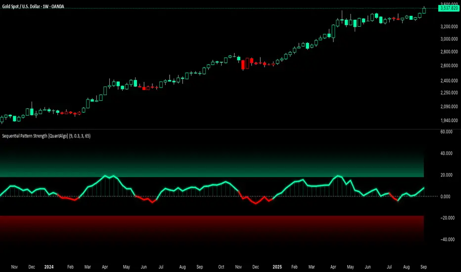
Sequential Pattern Strength [QuantAlgo]🟢 Overview
The Sequential Pattern Strength indicator measures the power and sustainability of consecutive price movements by tracking unbroken sequences of up or down closes. It incorporates sequence quality assessment, price extension analysis, and automatic exhaustion detection to help traders identify when strong trends are losing momentum and approaching potential reversal or continuation points.
🟢 How It Works
The indicator's key insight lies in its sequential pattern tracking system, where pattern strength is measured by analyzing consecutive price movements and their sustainability:
if close > close
upSequence := upSequence + 1
downSequence := 0
else if close < close
downSequence := downSequence + 1
upSequence := 0
The system calculates sequence quality by measuring how "perfect" the consecutive moves are:
perfectMoves = math.max(upSequence, downSequence)
totalMoves = math.abs(bar_index - ta.valuewhen(upSequence == 1 or downSequence == 1, bar_index, 0))
sequenceQuality = totalMoves > 0 ? perfectMoves / totalMoves : 1.0
First, it tracks price extension from the sequence starting point:
priceExtension = (close - sequenceStartPrice) / sequenceStartPrice * 100
Then, pattern exhaustion is identified when sequences become overextended:
isExhausted = math.abs(currentSequence) >= maxSequence or
math.abs(priceExtension) > resetThreshold * math.abs(currentSequence)
Finally, the pattern strength combines sequence length, quality, and price movement with momentum enhancement:
patternStrength = currentSequence * sequenceQuality * (1 + math.abs(priceExtension) / 10)
enhancedSignal = patternStrength + momentum * 10
signal = ta.ema(enhancedSignal, smooth)
This creates a sequence-based momentum indicator that combines consecutive movement analysis with pattern sustainability assessment, providing traders with both directional signals and exhaustion insights for entry/exit timing.
🟢 Signal Interpretation
Positive Values (Above Zero): Sequential pattern strength indicating bullish momentum with consecutive upward price movements and sustained buying pressure = Long/Buy opportunities
Negative Values (Below Zero): Sequential pattern strength indicating bearish momentum with consecutive downward price movements and sustained selling pressure = Short/Sell opportunities
Zero Line Crosses: Pattern transitions between bullish and bearish regimes, indicating potential trend changes or momentum shifts when sequences break
Upper Threshold Zone: Area above maximum sequence threshold (2x maxSequence) indicating extremely strong bullish patterns approaching exhaustion levels
Lower Threshold Zone: Area below negative threshold (-2x maxSequence) indicating extremely strong bearish patterns approaching exhaustion levels
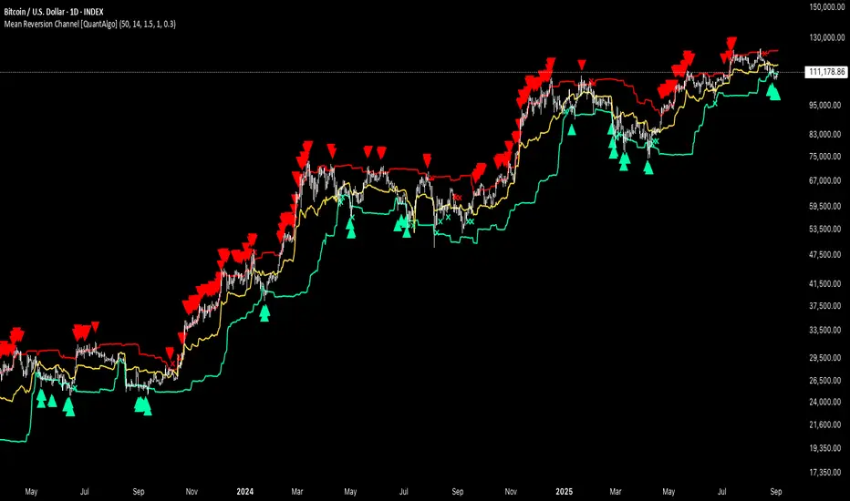
Mean Reversion Channel [QuantAlgo]🟢 Overview
The Mean Reversion Channel indicator is a range-bound trading system that combines dynamic price channels with momentum-weighted analysis to identify optimal mean reversion opportunities. It creates adaptive upper and lower reversion zones based on recent price action and volatility, while incorporating a momentum-biased equilibrium line that shifts based on volume-weighted price momentum. This creates a three-tier system where traders and investors can identify overbought and oversold conditions within established ranges, detect momentum exhaustion points, and anticipate channel breakouts or breakdowns. This indicator is particularly valuable for strategic dollar cost averaging (DCA) strategies, as it helps identify optimal accumulation zones during oversold conditions and provides tactical risk management levels for systematic investment approaches across different market conditions and asset classes.
🟢 How It Works
The indicator employs a four-stage calculation process that transforms raw price and volume data into actionable mean reversion signals. First, it establishes the base channel by calculating the highest high and lowest low over a user-defined lookback period, creating the foundational price range for mean reversion analysis. This channel adapts continuously as new price data becomes available, ensuring the system remains relevant to current market conditions.
In the second stage, the system calculates volume-weighted momentum by combining price momentum with volume activity. The momentum calculation takes the price change over a specified period and multiplies it by the volume ratio (current volume versus 20-period average volume, for instance) and a volume factor multiplier. This creates momentum readings that are more significant during high-volume periods and less influential during low-volume conditions.
The third stage creates the dynamic reversion zones using Average True Range (ATR) calculations. The upper reversion zone is positioned below the channel high by an ATR-based distance, while the lower reversion zone is positioned above the channel low. These zones contract when momentum is negative (upper zone) or positive (lower zone), creating asymmetric reversion bands that adapt to momentum conditions.
The final stage establishes the momentum-biased equilibrium line by calculating the midpoint between the reversion zones and adjusting it based on momentum bias. When momentum is positive, the equilibrium shifts upward; when negative, it shifts downward. This creates a dynamic reference level that helps identify when price action is moving against the prevailing momentum trend, signaling potential mean reversion opportunities.
🟢 How to Use
1. Mean Reversion Signal Identification
Lower Reversion Zone Signals: When price reaches or falls below the lower reversion zone with bearish momentum, the system generates potential long/buy entry signals indicating oversold conditions within the established range.
Upper Reversion Zone Signals: When price reaches or exceeds the upper reversion zone with bullish momentum, the system generates potential short/sell entry signals indicating overbought conditions.
2. Equilibrium Line Analysis and Momentum Exhaustion
Equilibrium Breaks: The dynamic equilibrium line serves as a momentum bias indicator within the channel. Price crossing above equilibrium suggests shifting to bullish bias, while breaks below indicate bearish bias development within the mean reversion framework.
Momentum Exhaustion Signals: The system identifies momentum exhaustion when price breaks through the equilibrium line opposite to the prevailing momentum direction. Bullish exhaustion occurs when price falls below equilibrium despite positive momentum, while bearish exhaustion happens when price rises above equilibrium during negative momentum periods.
3. Channel Expansion and Breakout Detection
Channel Boundary Breaks: When price breaks above the upper reversion zone or below the lower reversion zone, it signals potential channel expansion or false breakout conditions. These events often precede significant trend changes or range expansion phases.
Range Expansion Alerts: Breaks above the channel high or below the channel low indicate potential breakout from the mean reversion range, suggesting trend continuation or new directional movement beyond the established boundaries.
🟢 Pro Tips for Trading and Investing
→ Strategic DCA Optimization: Use the lower reversion zone as primary accumulation levels for dollar cost averaging strategies. When price reaches oversold conditions with bearish momentum exhaustion signals, it often represents optimal entry points for systematic investment programs, allowing investors to accumulate positions at statistically favorable price levels within the established range.
→ DCA Pause and Acceleration Signals : Monitor equilibrium line breaks to adjust DCA frequency and amounts. When price consistently trades below equilibrium with momentum exhaustion signals, consider accelerating DCA intervals or increasing investment amounts. Conversely, when price reaches upper reversion zones, consider pausing or reducing DCA activity until more favorable conditions return.
→ Momentum Divergence Detection: Watch for divergences between price action and momentum readings within the channel. When price makes new lows but momentum shows improvement, or price makes new highs with deteriorating momentum, these signal high-probability mean reversion setups ideal for contrarian investment approaches.
→ Alert-Based Systematic Investing/Trading: Utilize the comprehensive alert system for automated DCA triggers. Set up alerts for lower reversion zone touches combined with momentum exhaustion signals to create systematic entry points that remove emotional decision-making from long-term investment strategies, particularly effective for volatile assets where timing improvements can significantly impact overall returns.
Moving Average Adaptive RSI [BackQuant]Moving Average Adaptive RSI
What this is
A momentum oscillator that reshapes classic RSI into a zero-centered column plot and makes it adaptive. It builds RSI from two parts:
• A sensitivity window that scans several recent bars to capture the strongest up and down impulses.
• A selectable moving average that smooths those impulses before computing RSI.
The output ranges roughly from −100 to +100 with 0 as the midline, with optional extra smoothing and built-in divergence detection.
How it works
Impulse extraction
• For each bar the script inspects the last rsi_sen bars and collects upward and downward price changes versus the current price.
• It keeps the maximum upward change and maximum downward change from that window, emphasizing true bursts over single-bar noise.
MA-based averaging
• The up and down impulse series are averaged with your chosen MA over rsi_len bars.
• Supported MA types: SMA, EMA, DEMA, WMA, HMA, SMMA (RMA), TEMA.
Zero-centered RSI transform
• RS = UpMA ÷ DownMA, then mapped to a symmetric scale: 100 − 200 ÷ (1 + RS) .
• Above 0 implies positive momentum bias. Below 0 implies negative momentum bias.
Optional extra smoothing
• A second smoothing pass can be applied to the final oscillator using smoothing_len and smooth_type . Toggle with “Use Extra Smoothing”.
Visual encoding
• The oscillator is drawn as columns around the zero line with a gradient that intensifies toward extremes.
• Static bands mark 80 to 100 and −80 to −100 for extreme conditions.
Key inputs and what they change
• Price Source : input series for momentum.
• Calculation Period (rsi_len) : primary averaging window on up and down components. Higher = smoother, slower.
• Sensitivity (rsi_sen) : how many recent bars are scanned to find max impulses. Higher = more responsive to bursts.
• Calculation Type (ma_type) : MA family that shapes the core behavior. HMA or DEMA is faster, SMA or SMMA is slower.
• Smoothing Type and Length : optional second pass to calm noise on the final output.
• UI toggles : show or hide the oscillator, candle painting, and extreme bands.
Reading the oscillator
• Midline cross up (0) : momentum bias turning positive.
• Midline cross down (0) : momentum bias turning negative.
• Positive territory :
– 0 to 40: constructive but not stretched.
– 40 to 80: strong momentum, continuation more likely.
– Above 80: extreme risk of mean reversion grows.
• Negative territory : mirror the same levels for the downside.
Divergence detection
The script plots four divergence types using pivot highs and lows on both price and the oscillator. Lookbacks are set by lbL and lbR .
• Regular bullish : price lower low, oscillator higher low. Possible downside exhaustion.
• Hidden bullish : price higher low, oscillator lower low. Bias to trend continuation up.
• Regular bearish : price higher high, oscillator lower high. Possible upside exhaustion.
• Hidden bearish : price lower high, oscillator higher high. Bias to trend continuation down.
Labels: ℝ for regular, ℍ for hidden. Green for bullish, red for bearish.
Candle coloring
• Optional bar painting: green when the oscillator is above 0, red when below 0. This is for visual scanning only.
Strengths
• Adaptive sensitivity via a rolling impulse window that responds to genuine bursts.
• Configurable MA core so you can match responsiveness to the instrument.
• Zero-centered scale for simple regime reads with 0 as a clear bias line.
• Built-in regular and hidden divergence mapping.
• Flexible across symbols and timeframes once tuned.
Limitations and cautions
• Trends can remain extended. Treat extremes as context rather than automatic reversal signals.
• Divergence quality depends on pivot lookbacks. Short lookbacks give more signals with more noise. Long lookbacks reduce noise but add lag.
• Double smoothing can delay zero-line transitions. Balance smoothness and timeliness.
Practical usage ideas
• Regime filter : only take long setups from your separate method when the oscillator is above 0, shorts when below 0.
• Pullback confirmation : in uptrends, look for dips that hold above 0 or turn up from 0 to 40. Reverse for downtrends.
• Divergence as a heads-up : wait for a zero-line cross or a price trigger before acting on divergence.
• Sensitivity tuning : start with rsi_sen 2 to 5 on faster timeframes, increase slightly on slower charts.
Alerts
• MA-A RSI Long : oscillator crosses above 0.
• MA-A RSI Short : oscillator crosses below 0.
Use these as bias or timing aids, not standalone trade commands.
Settings quick reference
• Calculation : Price Source, Calculation Type, Calculation Period, Sensitivity.
• Smoothing : Smoothing Type, Smoothing Length, Use Extra Smoothing.
• UI : Show Oscillator, Paint Candles, Show Static High and Low Levels.
• Divergences : Pivot Lookback Left and Right, Div Signal Length, Show Detected Divergences.
Final thoughts
This tool reframes RSI by extracting strong short-term impulses and averaging them with a moving-average model of your choice, then presenting a zero-centered output for clear regime reads. Pair it with your structure, risk and execution process, and tune sensitivity and smoothing to the market you trade.

Hassi XAUUSD 15TF BUY/SELL (Anchored, Non-Repainting)What this does
Hassi XAUUSD 15TF BUY/SELL is a non-repainting signal indicator designed for XAUUSD (Gold) on the 15-minute timeframe (also works on BTCUSD). It blends EMA crossover + RSI + MACD with optional volume & volatility filters, and prints anchored BUY/SELL arrows that stay glued to their candle (no visual drifting on zoom/scale/replay). Optional confidence% labels help you judge signal quality at a glance.
Why it’s stable (no repaint)
Signals confirm only on bar close (barstate.isconfirmed).
Arrows/X marks are placed with label.new(x=bar_index, y=high/low, xloc.bar_index, yloc.abovebar/belowbar) so they remain exactly above/below the triggering candle.
No request.security for higher-TF lookaheads; no negative offsets.
How signals are generated
Core trigger: EMA(9) crosses EMA(21)
RSI filter (opt): RSI ≥ RSI Buy Min (default 50) for buys; ≤ RSI Sell Max (default 50) for sells
MACD filter (opt): MACD line crosses its signal or histogram sign matches direction
Volume/ATR filters (opt): require a basic volume spike and above-average ATR volatility (toggleable)
Divergence (opt): lightweight RSI divergence hints (diamond marks)
Anchored markers
BUY: triangle below the signal candle
SELL: triangle above the signal candle
EXIT (❌): small x above (long exit) / below (short exit) when the opposite signal confirms
Nudges: fine-tune vertical placement with tick offsets (inputs) without breaking anchoring
Inputs (defaults)
Fast EMA: 9
Slow EMA: 21
RSI Length: 14
MACD Fast/Slow/Signal: 12 / 26 / 9
Require RSI filter (50 line): ✅
Require MACD cross filter: ✅
RSI Buy Min / RSI Sell Max: 50 / 50
Buy/Sell/Exit Offset (ticks): 0 / 0 / 0
Advanced toggles: Trend Strength ✅, Dynamic Sizing (visual) ✅, Volume Filter ⛔, Volatility Filter ⛔, RSI Divergence ⛔, Show Confidence ✅
Status line/table: ✅
Alerts
Add any of these in Add Alert → Condition: this indicator
Buy Signal → {{ticker}} BUY @ {{close}} - ANCHORED SIGNAL
Sell Signal → {{ticker}} SELL @ {{close}} - ANCHORED SIGNAL
Exit Mark → {{ticker}} EXIT @ {{close}} - ANCHORED EXIT
Recommended use (15-minute XAUUSD)
Use during active sessions (London/NY overlaps).
Keep defaults; enable Volume & Volatility filters in high-noise conditions.
Add confluence (S/R, structure/BOS, session highs/lows, FVG or HTF bias).
Manage risk with structure-based SL or ATR x 1.0–1.5, and partial TP at 1:1–1.5R.
Note: You mentioned it has ~80% win rate on 15TF in your testing. Performance varies by broker feed, session, spread, and risk management. Treat results as educational, not a guarantee.
Non-repainting notes
Signals lock on close; historical arrows are final.
Labels are bar/price anchored (no drift when you zoom or change scale).
Arrays trim old labels automatically to avoid drawing limits.
FAQ
Q: Why don’t past arrows move when I resize the chart?
A: They’re label.new() anchored to bar_index and bar high/low with xloc/yloc, so they stay with the candle.
Q: Can I turn it into a strategy/backtest?
A: Yes—wrap the same signals into strategy.entry/exit, but this release is an indicator by design.
Q: Will it work on BTC or other pairs/timeframes?
A: Yes, but it’s tuned for XAUUSD M15. Adapt filters for other markets.
Changelog
v1.0 — Initial public release: anchored non-repainting arrows, optional RSI/MACD filters, volume/ATR filter, divergence hints, confidence labels, status panel, alerts.
Disclaimer
This tool is for education and analysis only. It is not financial advice. Trading involves risk; do your own research and manage risk responsibly.
PowerTrend Pro Strategy – Gold OptimizedTired of false signals on Gold?
PowerTrend Pro combines VWAP, Supertrend, RSI, and smart MA filters with trailing stops & break-even logic to deliver high-probability trades on XAUUSD.
PowerTrend Pro Strategy is a professional-grade trading system designed to capture high-probability swing and intraday opportunities on XAUUSD (Gold) and other volatile markets.
🔑 Core Features
VWAP Anchoring – institutional fair value reference to filter trades.
Supertrend (ATR-based) – adaptive trend filter tuned for Gold’s volatility.
Multi-Timeframe RSI – confirms momentum alignment across intraday and higher timeframe.
EMA + SMA Combo – ensures trades follow strong directional bias, reducing false signals.
Dynamic Risk Management
Adjustable Take Profit / Stop Loss (%)
Trailing Stop that locks in profits on extended moves
Break-Even Logic (stop loss moves to entry once price is in profit)
⚡ Gold-Tuned Presets
XAUUSD 1H → tighter TP/SL & faster entries for active intraday trading.
XAUUSD 4H → wider ATR filter & trailing stops to capture bigger swings.
Generic Mode → works on Forex, Indices, and Crypto (fully customizable).
🎯 Why It Works
Gold is notoriously volatile — quick spikes wipe out weak strategies. PowerTrend Pro solves this by combining:
✅ Institutional bias (VWAP)
✅ Adaptive trend filter (Supertrend)
✅ Momentum confirmation (RSI MTF)
✅ Robust trend structure (EMA + SMA)
✅ Smart exits (TP, SL, trailing & breakeven)
This multi-layer confirmation makes entries stronger and keeps risk under control.
🛠️ Usage
Add the strategy to your chart.
Choose a preset (XAUUSD 1H, 4H, or Generic).
Run Strategy Tester for performance metrics.
Optimize TP/SL and ATR values for your broker & market conditions.
🔥 Pro Tip: Combine this strategy with a session filter (London/NY overlap) or volume confirmation to boost accuracy in Gold.

Machine Learning BBPct [BackQuant]Machine Learning BBPct
What this is (in one line)
A Bollinger Band %B oscillator enhanced with a simplified K-Nearest Neighbors (KNN) pattern matcher. The model compares today’s context (volatility, momentum, volume, and position inside the bands) to similar situations in recent history and blends that historical consensus back into the raw %B to reduce noise and improve context awareness. It is informational and diagnostic—designed to describe market state, not to sell a trading system.
Background: %B in plain terms
Bollinger %B measures where price sits inside its dynamic envelope: 0 at the lower band, 1 at the upper band, ~ 0.5 near the basis (the moving average). Readings toward 1 indicate pressure near the envelope’s upper edge (often strength or stretch), while readings toward 0 indicate pressure near the lower edge (often weakness or stretch). Because bands adapt to volatility, %B is naturally comparable across regimes.
Why add (simplified) KNN?
Classic %B is reactive and can be whippy in fast regimes. The simplified KNN layer builds a “nearest-neighbor memory” of recent market states and asks: “When the market looked like this before, where did %B tend to be next bar?” It then blends that estimate with the current %B. Key ideas:
• Feature vector . Each bar is summarized by up to five normalized features:
– %B itself (normalized)
– Band width (volatility proxy)
– Price momentum (ROC)
– Volume momentum (ROC of volume)
– Price position within the bands
• Distance metric . Euclidean distance ranks the most similar recent bars.
• Prediction . Average the neighbors’ prior %B (lagged to avoid lookahead), inverse-weighted by distance.
• Blend . Linearly combine raw %B and KNN-predicted %B with a configurable weight; optional filtering then adapts to confidence.
This remains “simplified” KNN: no training/validation split, no KD-trees, no scaling beyond windowed min-max, and no probabilistic calibration.
How the script is organized (by input groups)
1) BBPct Settings
• Price Source – Which price to evaluate (%B is computed from this).
• Calculation Period – Lookback for SMA basis and standard deviation.
• Multiplier – Standard deviation width (e.g., 2.0).
• Apply Smoothing / Type / Length – Optional smoothing of the %B stream before ML (EMA, RMA, DEMA, TEMA, LINREG, HMA, etc.). Turning this off gives you the raw %B.
2) Thresholds
• Overbought/Oversold – Default 0.8 / 0.2 (inside ).
• Extreme OB/OS – Stricter zones (e.g., 0.95 / 0.05) to flag stretch conditions.
3) KNN Machine Learning
• Enable KNN – Switch between pure %B and hybrid.
• K (neighbors) – How many historical analogs to blend (default 8).
• Historical Period – Size of the search window for neighbors.
• ML Weight – Blend between raw %B and KNN estimate.
• Number of Features – Use 2–5 features; higher counts add context but raise the risk of overfitting in short windows.
4) Filtering
• Method – None, Adaptive, Kalman-style (first-order),
or Hull smoothing.
• Strength – How aggressively to smooth. “Adaptive” uses model confidence to modulate its alpha: higher confidence → stronger reliance on the ML estimate.
5) Performance Tracking
• Win-rate Period – Simple running score of past signal outcomes based on target/stop/time-out logic (informational, not a robust backtest).
• Early Entry Lookback – Horizon for forecasting a potential threshold cross.
• Profit Target / Stop Loss – Used only by the internal win-rate heuristic.
6) Self-Optimization
• Enable Self-Optimization – Lightweight, rolling comparison of a few canned settings (K = 8/14/21 via simple rules on %B extremes).
• Optimization Window & Stability Threshold – Governs how quickly preferred K changes and how sensitive the overfitting alarm is.
• Adaptive Thresholds – Adjust the OB/OS lines with volatility regime (ATR ratio), widening in calm markets and tightening in turbulent ones (bounded 0.7–0.9 and 0.1–0.3).
7) UI Settings
• Show Table / Zones / ML Prediction / Early Signals – Toggle informational overlays.
• Signal Line Width, Candle Painting, Colors – Visual preferences.
Step-by-step logic
A) Compute %B
Basis = SMA(source, len); dev = stdev(source, len) × multiplier; Upper/Lower = Basis ± dev.
%B = (price − Lower) / (Upper − Lower). Optional smoothing yields standardBB .
B) Build the feature vector
All features are min-max normalized over the KNN window so distances are in comparable units. Features include normalized %B, normalized band width, normalized price ROC, normalized volume ROC, and normalized position within bands. You can limit to the first N features (2–5).
C) Find nearest neighbors
For each bar inside the lookback window, compute the Euclidean distance between current features and that bar’s features. Sort by distance, keep the top K .
D) Predict and blend
Use inverse-distance weights (with a strong cap for near-zero distances) to average neighbors’ prior %B (lagged by one bar). This becomes the KNN estimate. Blend it with raw %B via the ML weight. A variance of neighbor %B around the prediction becomes an uncertainty proxy ; combined with a stability score (how long parameters remain unchanged), it forms mlConfidence ∈ . The Adaptive filter optionally transforms that confidence into a smoothing coefficient.
E) Adaptive thresholds
Volatility regime (ATR(14) divided by its 50-bar SMA) nudges OB/OS thresholds wider or narrower within fixed bounds. The aim: comparable extremeness across regimes.
F) Early entry heuristic
A tiny two-step slope/acceleration probe extrapolates finalBB forward a few bars. If it is on track to cross OB/OS soon (and slope/acceleration agree), it flags an EARLY_BUY/SELL candidate with an internal confidence score. This is explicitly a heuristic—use as an attention cue, not a signal by itself.
G) Informational win-rate
The script keeps a rolling array of trade outcomes derived from signal transitions + rudimentary exits (target/stop/time). The percentage shown is a rough diagnostic , not a validated backtest.
Outputs and visual language
• ML Bollinger %B (finalBB) – The main line after KNN blending and optional filtering.
• Gradient fill – Greenish tones above 0.5, reddish below, with intensity following distance from the midline.
• Adaptive zones – Overbought/oversold and extreme bands; shaded backgrounds appear at extremes.
• ML Prediction (dots) – The KNN estimate plotted as faint circles; becomes bright white when confidence > 0.7.
• Early arrows – Optional small triangles for approaching OB/OS.
• Candle painting – Light green above the midline, light red below (optional).
• Info panel – Current value, signal classification, ML confidence, optimized K, stability, volatility regime, adaptive thresholds, overfitting flag, early-entry status, and total signals processed.
Signal classification (informational)
The indicator does not fire trade commands; it labels state:
• STRONG_BUY / STRONG_SELL – finalBB beyond extreme OS/OB thresholds.
• BUY / SELL – finalBB beyond adaptive OS/OB.
• EARLY_BUY / EARLY_SELL – forecast suggests a near-term cross with decent internal confidence.
• NEUTRAL – between adaptive bands.
Alerts (what you can automate)
• Entering adaptive OB/OS and extreme OB/OS.
• Midline cross (0.5).
• Overfitting detected (frequent parameter flipping).
• Early signals when early confidence > 0.7.
These are purely descriptive triggers around the indicator’s state.
Practical interpretation
• Mean-reversion context – In range markets, adaptive OS/OB with ML smoothing can reduce whipsaws relative to raw %B.
• Trend context – In persistent trends, the KNN blend can keep finalBB nearer the mid/upper region during healthy pullbacks if history supports similar contexts.
• Regime awareness – Watch the volatility regime and adaptive thresholds. If thresholds compress (high vol), “OB/OS” comes sooner; if thresholds widen (calm), it takes more stretch to flag.
• Confidence as a weight – High mlConfidence implies neighbors agree; you may rely more on the ML curve. Low confidence argues for de-emphasizing ML and leaning on raw %B or other tools.
• Stability score – Rising stability indicates consistent parameter selection and fewer flips; dropping stability hints at a shifting backdrop.
Methodological notes
• Normalization uses rolling min-max over the KNN window. This is simple and scale-agnostic but sensitive to outliers; the distance metric will reflect that.
• Distance is unweighted Euclidean. If you raise featureCount, you increase dimensionality; consider keeping K larger and lookback ample to avoid sparse-neighbor artifacts.
• Lag handling intentionally uses neighbors’ previous %B for prediction to avoid lookahead bias.
• Self-optimization is deliberately modest: it only compares a few canned K/threshold choices using simple “did an extreme anticipate movement?” scoring, then enforces a stability regime and an overfitting guard. It is not a grid search or GA.
• Kalman option is a first-order recursive filter (fixed gain), not a full state-space estimator.
• Hull option derives a dynamic length from 1/strength; it is a convenience smoothing alternative.
Limitations and cautions
• Non-stationarity – Nearest neighbors from the recent window may not represent the future under structural breaks (policy shifts, liquidity shocks).
• Curse of dimensionality – Adding features without sufficient lookback can make genuine neighbors rare.
• Overfitting risk – The script includes a crude overfitting detector (frequent parameter flips) and will fall back to defaults when triggered, but this is only a guardrail.
• Win-rate display – The internal score is illustrative; it does not constitute a tradable backtest.
• Latency vs. smoothness – Smoothing and ML blending reduce noise but add lag; tune to your timeframe and objectives.
Tuning guide
• Short-term scalping – Lower len (10–14), slightly lower multiplier (1.8–2.0), small K (5–8), featureCount 3–4, Adaptive filter ON, moderate strength.
• Swing trading – len (20–30), multiplier ~2.0, K (8–14), featureCount 4–5, Adaptive thresholds ON, filter modest.
• Strong trends – Consider higher adaptive_upper/lower bounds (or let volatility regime do it), keep ML weight moderate so raw %B still reflects surges.
• Chop – Higher ML weight and stronger Adaptive filtering; accept lag in exchange for fewer false extremes.
How to use it responsibly
Treat this as a state descriptor and context filter. Pair it with your execution signals (structure breaks, volume footprints, higher-timeframe bias) and risk management. If mlConfidence is low or stability is falling, lean less on the ML line and more on raw %B or external confirmation.
Summary
Machine Learning BBPct augments a familiar oscillator with a transparent, simplified KNN memory of recent conditions. By blending neighbors’ behavior into %B and adapting thresholds to volatility regime—while exposing confidence, stability, and a plain early-entry heuristic—it provides an informational, probability-minded view of stretch and reversion that you can interpret alongside your own process.
Price Acceleration Matrix [QuantAlgo]🟢 Overview
The Price Acceleration Matrix indicator is an advanced momentum analysis tool that measures the rate of change in price velocity across multiple timeframes simultaneously. It transforms raw price data into velocity measurements for each timeframe, then calculates the acceleration of these velocities to identify when momentum is building or deteriorating. By analyzing acceleration alignment across all three timeframes, the system can distinguish between strong directional moves (all timeframes accelerating in the same direction) and weak, choppy movements (mixed acceleration signals). This multi-timeframe acceleration matrix provides traders with early warning signals for momentum shifts, trend continuation and reversal opportunities across different timeframes and asset classes.
🟢 How It Works
The indicator employs a three-stage calculation process that transforms price data into actionable acceleration signals. First, it calculates velocity (rate of price change) for each of the three user-defined timeframes by measuring the percentage change in price over the specified lookback periods. These velocity calculations are normalized by their respective timeframe lengths to ensure fair comparison across different periods.
In the second stage, the system calculates acceleration by measuring the change in velocity from one bar to the next for each timeframe, effectively capturing the second derivative of price movement. This acceleration data reveals whether momentum is building (positive acceleration) or deteriorating (negative acceleration) at each timeframe level.
The final stage creates the acceleration matrix score by evaluating alignment across all three timeframes. When all timeframes show positive acceleration, the system averages them for maximum bullish signal strength. When all show negative acceleration, it averages them for maximum bearish signal strength. However, when acceleration signals are mixed across timeframes, the system applies a penalty by dividing the average by two, indicating consolidation or conflicting momentum forces. The resulting signal is then smoothed using an Exponential Moving Average and scaled to the -3 to +3 range using a user-defined threshold parameter.
🟢 How to Use
1. Signal Interpretation and Momentum Analysis
Positive Territory (Above Zero): Indicates accelerating upward momentum with bullish bias and favorable conditions for long positions
Negative Territory (Below Zero): Signals accelerating downward momentum with bearish bias and favorable conditions for short positions
Extreme Levels (±2 to ±3): Represent maximum acceleration alignment across all timeframes, indicating high-probability momentum continuation
Moderate Levels (±1 to ±2): Suggest building momentum with good timeframe alignment but less conviction than extreme readings
Near Zero (-0.5 to +0.5): Indicates mixed signals, consolidation, or momentum exhaustion requiring caution
2. Overbought/Oversold Zone Analysis
Above +2 (Overbought Zone): Markets showing extreme bullish acceleration may be due for profit-taking or short-term pullbacks
Below -2 (Oversold Zone): Markets showing extreme bearish acceleration may present reversal opportunities or bounce potential
Zone Exits: When acceleration retreats from extreme zones, it often signals momentum exhaustion and potential trend changes
🟢 Pro Tips for Trading
→ Early Momentum Detection: Watch for acceleration crossing above zero after periods of negative readings, as this often precedes major price movements by several bars, providing early entry opportunities before traditional indicators signal.
→ Momentum Exhaustion Signals: Exit or take profits when acceleration reaches extreme levels (±2.5 or higher) and begins to decline, even if price continues in the same direction, as momentum deterioration typically precedes price reversals.
→ Acceleration Divergence Strategy: Look for divergences between price highs/lows and acceleration peaks/troughs, as these often signal weakening momentum and potential reversal opportunities before they become apparent on price charts.
→ Threshold Optimization: Adjust the acceleration threshold based on asset volatility - higher thresholds (0.7-1.0) for volatile assets to reduce false signals, lower thresholds (0.3-0.5) for stable assets to maintain sensitivity.
→ Alert-Based Trading: Utilize the built-in alert system for bullish/bearish reversals (±2 level crosses) and trend changes (zero line crosses) to capture momentum shifts without constant chart monitoring, especially effective for swing trading approaches.
→ Risk Management Integration: Reduce position sizes when acceleration readings are weak (below ±1.0) and increase allocation when strong acceleration alignment occurs (above ±2.0), as signal strength correlates directly with probability of successful trades.

Hassi XAUUSD Advanced FVG EMA/BOS/RSI/Volume + Session FilterWhat it does :
This strategy automates a popular ICT-style idea on XAUUSD (Gold): trade only when price taps back into a Fair Value Gap (FVG), but filter entries with trend, structure, momentum, volume, and session rules. It manages risk with fixed TP/SL (points) and shows a compact backtest panel on chart.
Core Logic
1) Market Structure (BOS)
Detects recent swing highs/lows and flags a Break of Structure:
BOS Up when price breaks the latest swing high.
BOS Down when price breaks the latest swing low.
2) FVG Detection (3-candle)
Bullish FVG when low > high and low > high .
Bearish FVG when high < low and high < low .
The most recent qualifying gap is drawn as a shaded box (optional).
3) Bias & Filters
Trend Bias: price vs EMA (default 200). Longs only above EMA; shorts only below.
Momentum: optional RSI filter (default 14); avoid longs in OB & shorts in OS.
Volume: optional filter requiring current volume > SMA(20) × multiplier.
Sessions: optional London / New York (PKT) time windows.
Entries & Exits
Long Entry (all must be true)
Above EMA, RSI bullish, volume ok, session ok, BOS Up.
A recent Bullish FVG exists (within N bars).
Price taps back into the FVG (low ≤ top & close > bottom) with a bullish candle.
Short Entry (mirror)
Below EMA, RSI bearish, volume ok, session ok, BOS Down.
A recent Bearish FVG exists (within N bars).
Price taps (high ≥ bottom & close < top) with a bearish candle.
Risk / R:R
Exits use fixed points on XAUUSD (default TP 100, SL 50).
On many gold feeds 1.0 = 10 points; inputs convert to price automatically.
“One-trade-at-a-time”: a new signal won’t fire until the previous position is flat.
Chart Labels
On entry, the script plots BUY/SELL plus fixed TP/SL lines & labels anchored to the entry bar (they don’t drift with price).
Visuals & Tools
EMA line (green/red by bias).
Swing points (tiny triangles) to see structure.
FVG boxes (green/red, optional).
Session shading (subtle blue overlay).
Stats Panel (top-right):
Total Trades, TP Hits, SL Hits, Win Rate, Profit Factor, Net P&L.
Inputs (quick guide)
EMA Length (default 200)
Swing Lookback for BOS (default 5)
FVG Box Length (how far the zone extends to the right)
TP / SL (points) for XAUUSD + display Risk:Reward
Sessions (PKT): London & New York windows + toggle
Filters: Volume (multiplier), RSI (length, OB/OS)
Visibility: show/hide FVG boxes & TP/SL drawings
Alerts
Buy Signal / Sell Signal on valid entries
Position Opened / Position Closed notifications
Best Practices & Notes
Designed for XAUUSD 15-minute. You can test other timeframes, but retune TP/SL points and filters accordingly.
Broker ticks differ: if your symbol steps are not 0.1, adjust TP/SL points.
Use with a HTF confluence (e.g., D1/4H bias, key S/R, news awareness).
Backtests are approximations; real results vary with spreads, slippage, and execution.
Disclaimer: This tool is for educational purposes. It is not financial advice. Always test before using on live capital.
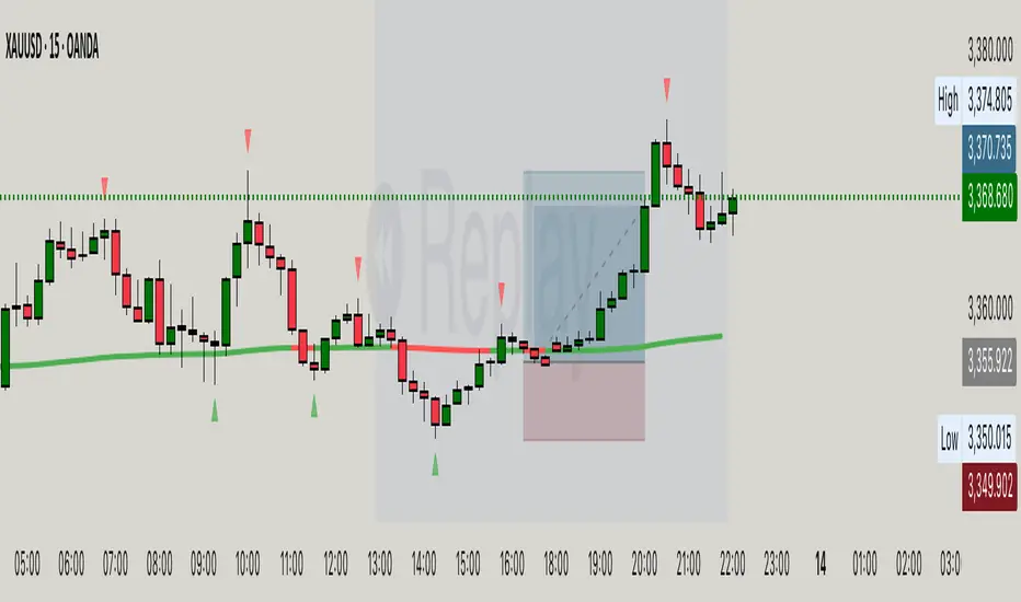
XAUUSD to GC1! ConverterThis simple utility indicator compares the spot gold price (XAUUSD) with the COMEX gold futures contract (GC1!).
It calculates the current spread between the two instruments and allows you to input a signal price on XAUUSD to instantly see the equivalent price on GC1!.
Perfect for traders who receive alerts on spot gold but execute on futures, ensuring seamless price adaptation.
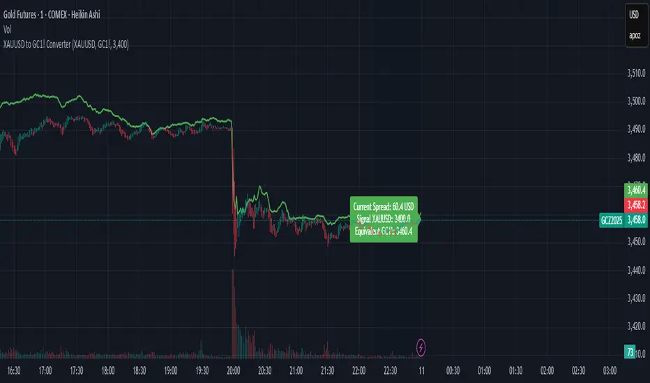
Hassi XAUUSD STRATEGY BOTGold (XAUUSD) 15m trend+momentum based signals with EMA(9/21/200), RSI, custom ADX, ATR-based SL/TP & alerts
Works on XAUUSD 15m.
Entry: EMA9/21 cross + price relative to EMA200 + RSI filter + custom ADX trend strength.
Risk: default SL=1.5×ATR, TP=2×ATR (editable).
Notes: No financial advice. Backtest before live use. Avoid high-impact news whipsaws.
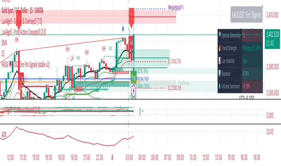
SD Bands Filtered Signals### SD Bands Filtered Signals: Reversion & Volatility Scanner
**Core Description:**
The SD Bands Filtered Signals is a tool developed to help traders identify more accurate buy and sell signals in sideways markets, or during periods of low price movement. It utilizes the principles of Standard Deviation (SD) and a Moving Average (MA), with a unique 'signal filtering' system added to reduce unnecessary noise.
**Key Features:**
* **SD Bands:** Creates upper and lower bands to define price volatility zones, providing a clear overview of market conditions.
* **Intelligent Reversal Signals:** Generates specially filtered Buy/Sell signals for a 'Reversion to the Mean' strategy. These signals appear only when the market has low volatility and the price touches the SD Bands.
* **Advanced Signal Filtering System:** Uses a **`Cooldown Bars`** variable to set a rest period between signals. This prevents repetitive arrows in the same zone, helping you find the best signal at the most suitable point.
* **Fully Customizable:** You can adjust the **`Length`**, **`Multiplier`**, **`Sideways Threshold`**, and **`Cooldown Bars`** to fit your trading style and asset of choice.
**How to Use:**
* **Buy Signal (Green Arrow Up):** Look for this signal when the market is sideways and the price moves down to touch the lower band (SD Low).
* **Sell Signal (Red Arrow Down):** Look for this signal when the market is sideways and the price moves up to touch the upper band (SD High).
* **Customization:** You can adjust the **`Cooldown Bars`** value to control the number of arrows. If you want more accurate but fewer signals, increase this value.
**Disclaimer:**
* This indicator is an **analytical tool only** and is not a 100% guarantee of profit.
* It should be used in conjunction with other forms of analysis, such as candlestick patterns, trading volume, and proper risk management.
ไทย
ชื่ออินดิเคเตอร์ "SD Bands Filtered Signals: Reversion & Volatility Scanner"
คำอธิบายหลัก:
อินดิเคเตอร์ SD Bands Filtered Signals เป็นเครื่องมือที่ถูกพัฒนาขึ้นเพื่อช่วยให้นักเทรดสามารถระบุสัญญาณซื้อ (Buy) และขาย (Sell) ที่แม่นยำขึ้นในตลาดแบบ Sideways หรือช่วงที่ราคาเคลื่อนที่ในกรอบแคบๆ โดยใช้หลักการของ Standard Deviation (SD) และ Moving Average (MA) และเพิ่มระบบ 'กรองสัญญาณ' ที่เป็นเอกลักษณ์เพื่อลดสัญญาณรบกวน (Noise) ที่ไม่จำเป็นออกไป
คุณสมบัติเด่น:
* SD Bands: สร้างเส้นขอบบนและล่างเพื่อระบุโซนความผันผวนของราคา ทำให้เห็นภาพรวมของตลาดได้ง่าย
* สัญญาณ Reversal อัจฉริยะ: สร้างสัญญาณ Buy/Sell ที่ถูกคัดกรองมาเป็นพิเศษสำหรับกลยุทธ์การกลับตัว (Reversion to the Mean) โดยจะปรากฏเฉพาะเมื่อตลาดมีความผันผวนต่ำและราคาแตะขอบของ SD Bands
* ระบบกรองสัญญาณขั้นสูง: ใช้ตัวแปร Cooldown Bars เพื่อกำหนดระยะเวลาพักสัญญาณ ทำให้ไม่เกิดลูกศรซ้ำๆ ในโซนเดียวกัน และช่วยให้คุณได้สัญญาณที่ดีที่สุดในจุดที่เหมาะสมที่สุด
* ปรับแต่งได้เต็มที่: คุณสามารถปรับค่า Length, Multiplier, Sideways Threshold และ Cooldown Bars เพื่อให้เข้ากับสไตล์การเทรดและคู่สินทรัพย์ที่คุณสนใจ
วิธีการใช้งาน:
* สัญญาณ Buy (ลูกศรสีเขียวขึ้น): มองหาสัญญาณนี้เมื่อตลาดอยู่ในช่วง Sideways และราคาวิ่งลงมาแตะเส้นขอบล่าง (SD Low)
* สัญญาณ Sell (ลูกศรสีแดงลง): มองหาสัญญาณนี้เมื่อตลาดอยู่ในช่วง Sideways และราคาวิ่งขึ้นไปแตะเส้นขอบบน (SD High)
* การปรับแต่ง: คุณสามารถปรับค่า Cooldown Bars เพื่อให้ได้จำนวนลูกศรที่ต้องการ หากต้องการสัญญาณที่แม่นยำขึ้นแต่จำนวนน้อยลง ให้เพิ่มค่านี้ให้สูงขึ้น
ข้อควรระวัง:
* อินดิเคเตอร์นี้เป็นเพียงเครื่องมือวิเคราะห์ ไม่ใช่สัญญาณที่การันตีผลกำไร 100%
* ควรใช้ประกอบกับการวิเคราะห์อื่นๆ เช่น รูปแบบแท่งเทียน, ปริมาณการซื้อขาย (Volume) และการจัดการความเสี่ยงที่เหมาะสม
