[e2] Drawing Library :: Horizontal Ray█ OVERVIEW
Library "e2hray"
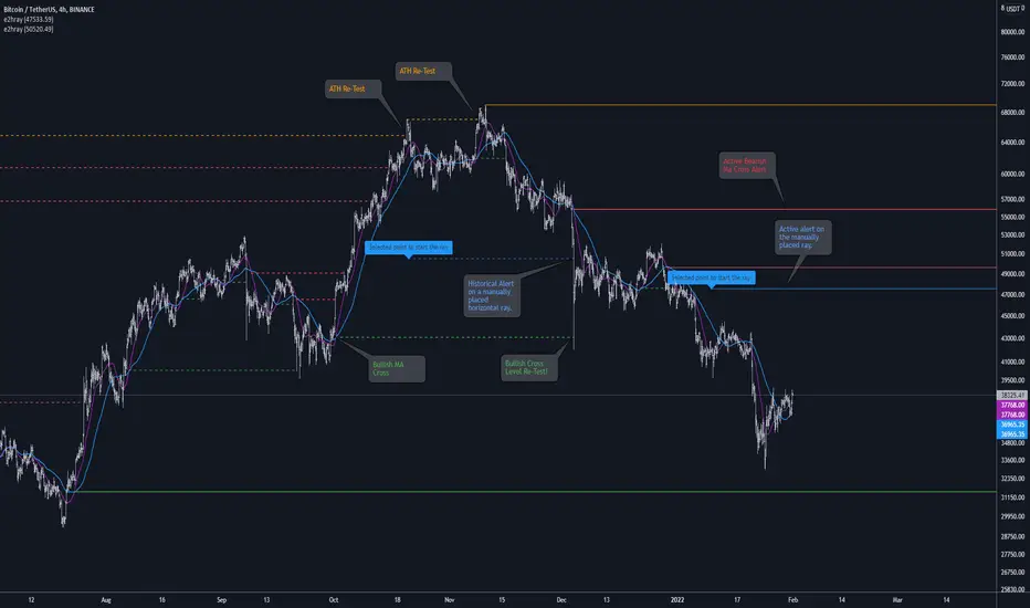
A drawing library that contains the hray() function, which draws a horizontal ray/s with an initial point determined by a specified condition. It plots a ray until it reached the price. The function let you control the visibility of historical levels and setup the alerts.
█ HORIZONTAL RAY FUNCTION
hray(condition, level, color, extend, hist_lines, alert_message, alert_delay, style, hist_style, width, hist_width)
Parameters:
condition : Boolean condition that defines the initial point of a ray
level : Ray price level.
color : Ray color.
extend : (optional) Default value true, current ray levels extend to the right, if false - up to the current bar.
hist_lines : (optional) Default value true, shows historical ray levels that were revisited, default is dashed lines. To avoid alert problems set to 'false' before creating alerts.
alert_message : (optional) Default value string(na), if declared, enables alerts that fire when price revisits a line, using the text specified
alert_delay : (optional) Default value int(0), number of bars to validate the level. Alerts won't trigger if the ray is broken during the 'delay'.
style : (optional) Default value 'line.style_solid'. Ray line style.
hist_style : (optional) Default value 'line.style_dashed'. Historical ray line style.
width : (optional) Default value int(1), ray width in pixels.
hist_width : (optional) Default value int(1), historical ray width in pixels.
Returns: void
█ EXAMPLES
• Example 1. Single horizontal ray from the dynamic input.
//@version=5
indicator("hray() example :: Dynamic input ray", overlay = true)
import e2e4mfck/e2hray/1 as e2draw
inputTime = input.time(timestamp("20 Jul 2021 00:00 +0300"), "Date", confirm = true)
inputPrice = input.price(54, 'Price Level', confirm = true)
e2draw.hray(time == inputTime, inputPrice, color.blue, alert_message = 'Ray level re-test!')
var label mark = label.new(inputTime, inputPrice, 'Selected point to start the ray', xloc.bar_time)
• Example 2. Multiple horizontal rays on the moving averages cross.
//@version=5
indicator("hray() example :: MA Cross", overlay = true)
import e2e4mfck/e2hray/1 as e2draw
float sma1 = ta.sma(close, 20)
float sma2 = ta.sma(close, 50)
bullishCross = ta.crossover( sma1, sma2)
bearishCross = ta.crossunder(sma1, sma2)
plot(sma1, 'sma1', color.purple)
plot(sma2, 'sma2', color.blue)
// 1a. We can use 2 function calls to distinguish long and short sides.
e2draw.hray(bullishCross, sma1, color.green, alert_message = 'Bullish Cross Level Broken!', alert_delay = 10)
e2draw.hray(bearishCross, sma2, color.red, alert_message = 'Bearish Cross Level Broken!', alert_delay = 10)
// 1b. Or a single call for both.
// e2draw.hray(bullishCross or bearishCross, sma1, bullishCross ? color.green : color.red)
• Example 3. Horizontal ray at the all time highs with an alert.
//@version=5
indicator("hray() example :: ATH", overlay = true)
import e2e4mfck/e2hray/1 as e2draw
var float ath = 0, ath := math.max(high, ath)
bool newAth = ta.change(ath)
e2draw.hray(nz(newAth ), high , color.orange, alert_message = 'All Time Highs Tested!', alert_delay = 10)
Wyszukaj w skryptach "VAR+计量模型+黄金期货"
Moving Average Multitool CrossoverAs per request, this is a moving average crossover version of my original moving average multitool script .
It allows you to easily access and switch between different types of moving averages, without having to continuously add and remove different moving averages from your chart. This should make backtesting moving average crossovers much, much more easier. It also has the option to show buy and sell signals for the crossovers of the chosen moving averages.
It contains the following moving averages:
Exponential Moving Average (EMA)
Simple Moving Average (SMA)
Weighted Moving Average (WMA)
Double Exponential Moving Average (DEMA)
Triple Exponential Moving Average (TEMA)
Triangular Moving Average (TMA)
Volume-Weighted Moving Average (VWMA)
Smoothed Moving Average (SMMA)
Hull Moving Average (HMA)
Least Squares Moving Average (LSMA)
Kijun-Sen line from the Ichimoku Kinko-Hyo system (Kijun)
McGinley Dynamic (MD)
Rolling Moving Average (RMA)
Jurik Moving Average (JMA)
Arnaud Legoux Moving Average (ALMA)
Vector Autoregression Moving Average (VAR)
Welles Wilder Moving Average (WWMA)
Sine Weighted Moving Average (SWMA)
Leo Moving Average (LMA)
Variable Index Dynamic Average (VIDYA)
Fractal Adaptive Moving Average (FRAMA)
Variable Moving Average (VAR)
Geometric Mean Moving Average (GMMA)
Corrective Moving Average (CMA)
Moving Median (MM)
Quick Moving Average (QMA)
Kaufman's Adaptive Moving Average (KAMA)
Volatility-Adjusted Moving Average (VAMA)
Modular Filter (MF)

benchLibrary "bench"
A simple banchmark library to analyse script performance and bottlenecks.
Very useful if you are developing an overly complex application in Pine Script, or trying to optimise a library / function / algorithm...
Supports artificial looping benchmarks (of fast functions)
Supports integrated linear benchmarks (of expensive scripts)
One important thing to note is that the Pine Script compiler will completely ignore any calculations that do not eventually produce chart output. Therefore, if you are performing an artificial benchmark you will need to use the bench.reference(value) function to ensure the calculations are executed.
Please check the examples towards the bottom of the script.
Quick Reference
(Be warned this uses non-standard space characters to get the line indentation to work in the description!)
```
// Looping benchmark style
benchmark = bench.new(samples = 500, loops = 5000)
data = array.new_int()
if bench.start(benchmark)
while bench.loop(benchmark)
array.unshift(data, timenow)
bench.mark(benchmark)
while bench.loop(benchmark)
array.unshift(data, timenow)
bench.mark(benchmark)
while bench.loop(benchmark)
array.unshift(data, timenow)
bench.stop(benchmark)
bench.reference(array.get(data, 0))
bench.report(benchmark, '1x array.unshift()')
// Linear benchmark style
benchmark = bench.new()
data = array.new_int()
bench.start(benchmark)
for i = 0 to 1000
array.unshift(data, timenow)
bench.mark(benchmark)
for i = 0 to 1000
array.unshift(data, timenow)
bench.stop(benchmark)
bench.reference(array.get(data, 0))
bench.report(benchmark,'1000x array.unshift()')
```
Detailed Interface
new(samples, loops) Initialises a new benchmark array
Parameters:
samples : int, the number of bars in which to collect samples
loops : int, the number of loops to execute within each sample
Returns: int , the benchmark array
active(benchmark) Determing if the benchmarks state is active
Parameters:
benchmark : int , the benchmark array
Returns: bool, true only if the state is active
start(benchmark) Start recording a benchmark from this point
Parameters:
benchmark : int , the benchmark array
Returns: bool, true only if the benchmark is unfinished
loop(benchmark) Returns true until call count exceeds bench.new(loop) variable
Parameters:
benchmark : int , the benchmark array
Returns: bool, true while looping
reference(number, string) Add a compiler reference to the chart so the calculations don't get optimised away
Parameters:
number : float, a numeric value to reference
string : string, a string value to reference
mark(benchmark, number, string) Marks the end of one recorded interval and the start of the next
Parameters:
benchmark : int , the benchmark array
number : float, a numeric value to reference
string : string, a string value to reference
stop(benchmark, number, string) Stop the benchmark, ending the final interval
Parameters:
benchmark : int , the benchmark array
number : float, a numeric value to reference
string : string, a string value to reference
report(Prints, benchmark, title, text_size, position)
Parameters:
Prints : the benchmarks results to the screen
benchmark : int , the benchmark array
title : string, add a custom title to the report
text_size : string, the text size of the log console (global size vars)
position : string, the position of the log console (global position vars)
unittest_bench(case) Cache module unit tests, for inclusion in parent script test suite. Usage: bench.unittest_bench(__ASSERTS)
Parameters:
case : string , the current test case and array of previous unit tests (__ASSERTS)
unittest(verbose) Run the bench module unit tests as a stand alone. Usage: bench.unittest()
Parameters:
verbose : bool, optionally disable the full report to only display failures

logLibrary "log"
Logging library for easily displaying debug, info, warn, error and critical messages.
No real need to explain why you might want to use this library! I'm sure you've all experienced the frustration of trying to understand the data state of your scripts... so, enjoy! More on it's way...
(Don't forget to check the helpers in the script and the useful tips below)
Some Useful Tips
By default the log console persists between bars (for history) and bars and ticks (for realtime).
Sometimes it is useful to clear the log after each candle or tick (assuming we are using the above helpers):
```
log_print(clear = true) // starts afresh on every bar and tick (excludes historical bars but good realtime tick analysis)
log_print(clear = barstate.isnew) // clears the log at the start of each bar (again, excludes historical but good realtime candle analysis)
```
It is also useful to be able to selectively understand the state of data at specific points or times within a script:
```
if log.once()
debug('useful variable', my_var) // this log only gets written once, upon first execution of this statement
if log.only(5)
debug3(a, b, c) // these variables are only logged the first five times this statement is executed
log_print(clear = false) // clear must be false and you should not write other logs on every bar, or the above will be lost
```
Final tip. If you want to view ONLY log entries of a particular level, then negate the constant:
```
log_print(level = -LOG_DEBUG)
```
Detailed Interface
once() Restrict execution to only happen once. Usage: if assert.once()\n happens_once()
Returns: bool, true on first execution within scope, false subsequently
only(repeat) Restrict execution to happen a set number of times. Usage: if assert.only(5)\n happens_five_times()
Parameters:
repeat : int, the number of times to return true
Returns: bool, true for the set number of times within scope, false subsequently
init() Initialises the log array
Returns: string , tuple based array to contain all pending log entries (__LOG)
clear(msgs) Clears the log array
Parameters:
msgs : string , the current collection of unfiltered and unprocessed logs (__LOG)
trace(msgs, msg) Writes a trace message to the log console
Parameters:
msgs : string , the current collection of unfiltered and unprocessed logs (__LOG)
msg : string, the trace message to write to the log
debug(msgs, msg) Writes a debug message to the log console
Parameters:
msgs : string , the current collection of unfiltered and unprocessed logs (__LOG)
msg : string, the debug message to write to the log
info(msgs, msg) Writes an info message to the log console
Parameters:
msgs : string , the current collection of unfiltered and unprocessed logs (__LOG)
msg : string, the info message to write to the log
warn(msgs, msg) Writes a warning message to the log console
Parameters:
msgs : string , the current collection of unfiltered and unprocessed logs (__LOG)
msg : string, the warn message to write to the log
error(msgs, msg) Writes an error message to the log console
Parameters:
msgs : string , the current collection of unfiltered and unprocessed logs (__LOG)
msg : string, the error message to write to the log
fatal(msgs, msg) Writes a critical message to the log console
Parameters:
msgs : string , the current collection of unfiltered and unprocessed logs (__LOG)
msg : string, the fatal message to write to the log
log(msgs, level, msg) Write a log message to the log console with a custom level
Parameters:
msgs : string , the current collection of unfiltered and unprocessed logs (__LOG)
level : ing, the logging level to assign to the message
msg : string, the log message to write to the log
severity(msgs) Checks the unprocessed log messages and returns the highest present level
Parameters:
msgs : string , the current collection of unfiltered and unprocessed logs (__LOG)
Returns: int, the highest level found within the unfiltered logs
print(msgs, level, clear, rows, text_size, position) Prints all log messages to the screen
Parameters:
msgs : string , the current collection of unfiltered and unprocessed logs (__LOG)
level : int, the minimum required log level of each message to be displayed
clear : bool, clear the printed log console after each render (useful with realtime when set to barstate.isconfirmed)
rows : int, the number of rows to display in the log console
text_size : string, the text size of the log console (global size vars)
position : string, the position of the log console (global position vars)
unittest_log(case) Log module unit tests, for inclusion in parent script test suite. Usage: log.unittest_log(__ASSERTS)
Parameters:
case : string , the current test case and array of previous unit tests (__ASSERTS)
unittest(verbose) Run the log module unit tests as a stand alone. Usage: log.unittest()
Parameters:
verbose : bool, optionally disable the full report to only display failures

CreateAndShowZigzagLibrary "CreateAndShowZigzag"
Functions in this library creates/updates zigzag array and shows the zigzag
getZigzag(zigzag, prd, max_array_size) calculates zigzag using period
Parameters:
zigzag : is the float array for the zigzag (should be defined like "var zigzag = array.new_float(0)"). each zigzag points contains 2 element: 1. price level of the zz point 2. bar_index of the zz point
prd : is the length to calculate zigzag waves by highest(prd)/lowest(prd)
max_array_size : is the maximum number of elements in zigzag, keep in mind each zigzag point contains 2 elements, so for example if it's 10 then zigzag has 10/2 => 5 zigzag points
Returns: dir that is the current direction of the zigzag
showZigzag(zigzag, oldzigzag, dir, upcol, dncol) this function shows zigzag
Parameters:
zigzag : is the float array for the zigzag (should be defined like "var zigzag = array.new_float(0)"). each zigzag points contains 2 element: 1. price level of the zz point 2. bar_index of the zz point
oldzigzag : is the float array for the zigzag, you get copy the zigzag array to oldzigzag by "oldzigzag = array.copy(zigzay)" before calling get_zigzag() function
dir : is the direction of the zigzag wave
upcol : is the color of the line if zigzag direction is up
dncol : is the color of the line if zigzag direction is down
Returns: null
Profit Maximizer StrategyFirst I would like to thank to @KivancOzbilgic for developing this indicator.
All the credit goes to him.
I just created a strategy, in order to try to find the perfect parameters, timeframe and currency for it.
I will provide below the same description like he has in the publish of profit maximizer
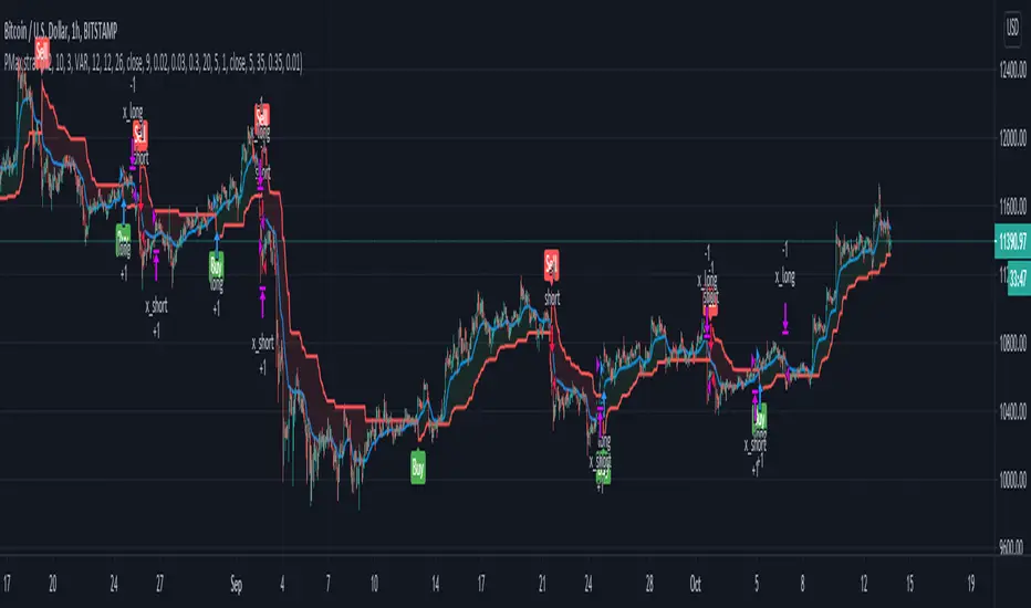
Profit Maximizer - PMax combines the powerful sides of MOST (Moving Average Trend Changer) and SuperTrend (ATR price detection) in one indicator.
Backtest and optimization results of PMax are far better when compared to its ancestors MOST and SuperTrend. It reduces the number of false signals in sideways and give more reliable trade signals.
PMax is easy to determine the trend and can be used in any type of markets and instruments. It does not repaint.
The first parameter in the PMax indicator set by the three parameters is the period/length of ATR.
The second Parameter is the Multiplier of ATR which would be useful to set the value of distance from the built in Moving Average.
I personally think the most important parameter is the Moving Average Length and type.
PMax will be much sensitive to trend movements if Moving Average Length is smaller. And vice versa, will be less sensitive when it is longer.
As the period increases it will become less sensitive to little trends and price actions.
In this way, your choice of period, will be closely related to which of the sort of trends you are interested in.
We are under the effect of the uptrend in cases where the Moving Average is above PMax;
conversely under the influence of a downward trend, when the Moving Average is below PMax.
Built in Moving Average type defaultly set as EMA but users can choose from 8 different Moving Average types like:
SMA : Simple Moving Average
EMA : Exponential Movin Average
WMA : Weighted Moving Average
TMA : Triangular Moving Average
VAR : Variable Index Dynamic Moving Average aka VIDYA
WWMA : Welles Wilder's Moving Average
ZLEMA : Zero Lag Exponential Moving Average
TSF : True Strength Force
Tip: In sideways VAR would be a good choice
You can use PMax default alarms and Buy Sell signals like:
1-
BUY when Moving Average crosses above PMax
SELL when Moving Average crosses under PMax
2-
BUY when prices jumps over PMax line.
SELL when prices go under PMax line.
PMax Explorer STRATEGY & SCREENERProfit Maximizer - PMax Explorer STRATEGY & SCREENER screens the BUY and SELL signals (trend reversals) for 20 user defined different tickers in Tradingview charts.
Simply input the name of the ticker in Tradingview that you want to screen.
Terminology explanation:
Confirmed Reversal: PMax reversal that happened in the last bar and cannot be repainted.
Potential Reversal: PMax reversal that might happen in the current bar but can also not happen depending upon the timeframe closing price.
Downtrend: Tickers that are currently in the sell zone
Uptrend: Tickers that are currently in the buy zone
Screener has also got a built in PMax indicator which users can confirm the reversals on graphs.
Screener explores the 20 tickers in current graph's time frame and also in desired parameters of the SuperTrend indicator.
Also you can optimize the parameters manually with the built in STRATEGY version.
PMax indicator :
Profit Maximizer - PMax is a brand new indicator developed by me.
It's a combination of two trailing stop loss indicators;
One is Anıl Özekşi's MOST (Moving Stop Loss) Indicator
and the other one is well known ATR based SuperTrend
Profit Maximizer - PMax tries to solve this problem. PMax combines the powerful sides of MOST (Moving Average Trend Changer) and SuperTrend (ATR price detection) in one indicator.
Backtest and optimization results of PMax are far better when compared to its ancestors MOST and SuperTrend. It reduces the number of false signals in sideways and give more reliable trade signals.
PMax is easy to determine the trend and can be used in any type of markets and instruments. It does not repaint.
The first parameter in the PMax indicator set by the three parameters is the period/length of ATR.
The second Parameter is the Multiplier of ATR which would be useful to set the value of distance from the built in Moving Average.
I personally think the most important parameter is the Moving Average Length and type.
PMax will be much sensitive to trend movements if Moving Average Length is smaller. And vice versa, will be less sensitive when it is longer.
As the period increases it will become less sensitive to little trends and price actions.
In this way, your choice of period, will be closely related to which of the sort of trends you are interested in.
We are under the effect of the uptrend in cases where the Moving Average is above PMax;
conversely under the influence of a downward trend, when the Moving Average is below PMax.
Built in Moving Average type defaultly set as EMA but users can choose from 8 different Moving Average types like:
SMA : Simple Moving Average
EMA : Exponential Movin Average
WMA : Weighted Moving Average
TMA : Triangular Moving Average
VAR : Variable Index Dynamic Moving Average aka VIDYA
WWMA : Welles Wilder's Moving Average
ZLEMA : Zero Lag Exponential Moving Average
TSF : True Strength Force
Tip: In sideways VAR would be a good choice
You can use PMax default alarms and Buy Sell signals like:
1-
BUY when Moving Average crosses above PMax
SELL when Moving Average crosses under PMax
2-
BUY when prices jumps over PMax line.
SELL when prices go under PMax line.

Profit Maximizer PMaxPMax is a brand new indicator developed by KivancOzbilgic in earlier 2020.
It's a combination of two trailing stop loss indicators;
One is Anıl Özekşi's MOST (Moving Stop Loss) Indicator
and the other one is well known ATR based SuperTrend.
Both MOST and SuperTrend Indicators are very good at trend following systems but conversely their performance is not bright in sideways market conditions like most of the other indicators.
Profit Maximizer - PMax tries to solve this problem. PMax combines the powerful sides of MOST (Moving Average Trend Changer) and SuperTrend (ATR price detection) in one indicator.
Backtest and optimization results of PMax are far better when compared to its ancestors MOST and SuperTrend. It reduces the number of false signals in sideways and give more reliable trade signals.
PMax is easy to determine the trend and can be used in any type of markets and instruments. It does not repaint.
The first parameter in the PMax indicator set by the three parameters is the period/length of ATR.
The second Parameter is the Multiplier of ATR which would be useful to set the value of distance from the built in Moving Average.
I personally think the most important parameter is the Moving Average Length and type.
PMax will be much sensitive to trend movements if Moving Average Length is smaller. And vice versa, will be less sensitive when it is longer.
As the period increases it will become less sensitive to little trends and price actions.
In this way, your choice of period, will be closely related to which of the sort of trends you are interested in.
We are under the effect of the uptrend in cases where the Moving Average is above PMax;
conversely under the influence of a downward trend, when the Moving Average is below PMax.
Built in Moving Average type defaultly set as EMA but users can choose from 8 different Moving Average types like:
SMA : Simple Moving Average
EMA : Exponential Movin Average
WMA : Weighted Moving Average
TMA : Triangular Moving Average
VAR : Variable Index Dynamic Moving Average aka VIDYA
WWMA : Welles Wilder's Moving Average
ZLEMA : Zero Lag Exponential Moving Average
TSF : True Strength Force
Tip: In sideways VAR would be a good choice
You can use PMax default alarms and Buy Sell signals like:
1-
BUY when Moving Average crosses above PMax
SELL when Moving Average crosses under PMax
2-
BUY when prices jumps over PMax line.
SELL when prices go under PMax line.

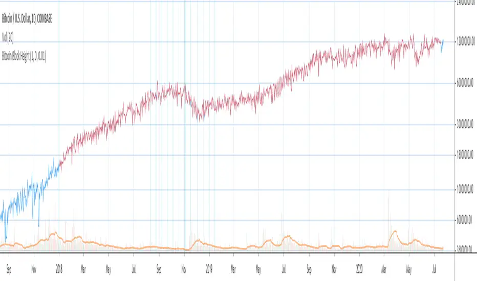
Bitcoin Block Height (Total Blocks)Bitcoin Block Height by RagingRocketBull 2020
Version 1.0
Differences between versions are listed below:
ver 1.0: compare QUANDL Difficulty vs Blockchain Difficulty sources, get total error estimate
ver 2.0: compare QUANDL Hash Rate vs Blockchain Hash Rate sources, get total error estimate
ver 3.0: Total Blocks estimate using different methods
--------------------------------
This indicator estimates Bitcoin Block Height (Total Blocks) using Difficulty and Hash Rate in the most accurate way possible, since
QUANDL doesn't provide a direct source for Bitcoin Block Height (neither QUANDL:BCHAIN, nor QUANDL:BITCOINWATCH/MINING).
Bitcoin Block Height can be used in other calculations, for instance, to estimate the next date of Bitcoin Halving.
Using this indicator I demonstrate:
- that QUANDL data is not accurate and differ from Blockchain source data (industry standard), but still can be used in calculations
- how to plot a series of data points from an external csv source and compare it with another source
- how to accurately estimate Bitcoin Block Height
Features:
- compare QUANDL Difficulty source (EOD, D1) with external Blockchain Difficulty csv source (EOD, D1, embedded)
- show/hide Quandl/Blockchain Difficulty curves
- show/hide Blockchain Difficulty candles
- show/hide differences (aqua vertical lines)
- show/hide time gaps (green vertical lines)
- count source differences within data range only or for the whole history
- multiply both sources by alpha to match before comparing
- floor/round both matched sources when comparing
- Blockchain Difficulty offset to align sequences, bars > 0
- count time gaps and missing bars (as result of time gaps)
WARNING:
- This indicator hits the max 1000 vars limit, adding more plots/vars/data points is not possible
- Both QUANDL/Blockchain provide daily EOD data and must be plotted on a daily D1 chart otherwise results will be incorrect
- current chart must not have any time gaps inside the range (time gaps outside the range don't affect the calculation). Time gaps check is provided.
Otherwise hardcoded Blockchain series will be shifted forward on gaps and the whole sequence become truncated at the end => data comparison/total blocks estimate will be incorrect
Examples of valid charts that can run this indicator: COINBASE:BTCUSD,D1 (has 8 time gaps, 34 missing bars outside the range), QUANDL:BCHAIN/DIFF,D1 (has no gaps)
Usage:
- Description of output plot values from left to right:
- c_shifted - 4x blockchain plotcandles ohlc, green/black (default na)
- diff - QUANDL Difficulty
- c_shifted - Blockchain Difficulty with offset
- QUANDL Difficulty multiplied by alpha and rounded
- Blockchain Difficulty multiplied by alpha and rounded
- is_different, bool - cur bar's source values are different (1) or not (0)
- count, number of differences
- bars, total number of bars/data points in the range
- QUANDL daily blocks
- Blockchain daily blocks
- QUANDL total blocks
- Blockchain total blocks
- total_error - difference between total_blocks estimated using both sources as of cur bar, blocks
- number_of_gaps - number of time gaps on a chart
- missing_bars - number of missing bars as result of time gaps on a chart
- Color coding:
- Blue - QUANDL data
- Red - Blockchain data
- Black - Is Different
- Aqua - number of differences
- Green - number of time gaps
- by default the indicator will show lots of vertical aqua lines, 138 differences, 928 bars, total error -370 blocks
- to compare the best match of the 2 sources shift Blockchain source 1 bar into the future by setting Blockchain Difficulty offset = 1, leave alpha = 0.01 =>
this results in no vertical aqua lines, 0 differences, total_error = 0 blocks
if you move the mouse inside the range some bars will show total_error = 1 blocks => total_error <= 1 blocks
- now uncheck Round Difficulty Values flag => some filled aqua areas, 218 differences.
- now set alpha = 1 (use raw source values) instead of 0.01 => lots of filled aqua areas, 871 differences.
although there are many differences this still doesn't affect the total_blocks estimate provided Difficulty offset = 1
Methodology:
To estimate Bitcoin Block Height we need 3 steps, each step has its own version:
- Step 1: Compare QUANDL Difficulty vs Blockchain Difficulty sources and estimate error based on differences
- Step 2: Compare QUANDL Hash Rate vs Blockchain Hash Rate sources and estimate error based on differences
- Step 3: Estimate Bitcoin Block Height (Total Blocks) using different methods in the most accurate way possible
QUANDL doesn't provide block time data, but we can calculate it using the Hash Rate approximation formula:
estimated Hash rate/sec H = 2^32 * D / T, where D - Difficulty, T - block time, sec
1. block time (T) can be derived from the formula, since we already know Difficulty (D) and Hash Rate (H) from QUANDL
2. using block time (T) we can estimate daily blocks as daily time / block time
3. block height (total blocks) = cumulative sum of daily blocks of all bars on the chart (that's why having no gaps is important)
Notes:
- This code uses Pinescript v3 compatibility framework
- hash rate is in THash/s, although QUANDL falsely states in description GHash/s! THash = 1000 GHash
- you can't read files, can only embed/hardcode raw data in script
- both QUANDL and Blockchain sources have no gaps
- QUANDL and Blockchain series are different in the following ways:
- all QUANDL data is already shifted 1 bar into the future, i.e. prev day's value is shown as cur day's value => Blockchain data must be shifted 1 bar forward to match
- all QUANDL diff data > 1 bn (10^12) are truncated and have last 1-2 digits as zeros, unlike Blockchain data => must multiply both values by 0.01 and floor/round the results
- QUANDL sometimes rounds, other times truncates those 1-2 last zero digits to get the 3rd last digit => must use both floor/round
- you can only shift sequences forward into the future (right), not back into the past (left) using positive offset => only Blockchain source can be shifted
- since total_blocks is already a cumulative sum of all prev values on each bar, total_error must be simple delta, can't be also int(cum()) or incremental
- all Blockchain values and total_error are na outside the range - move you mouse cursor on the last bar/inside the range to see them
TLDR, ver 1.0 Conclusion:
QUANDL/Blockchain Difficulty source differences don't affect total blocks estimate, total error <= 1 block with avg 150 blocks/day is negligible
Both QUANDL/Blockchain Difficulty sources are equally valid and can be used in calculations. QUANDL is a relatively good stand in for Blockchain industry standard data.
Links:
QUANDL difficulty source: www.quandl.com
QUANDL hash rate source: www.quandl.com
Blockchain difficulty source (export data as csv): www.blockchain.com
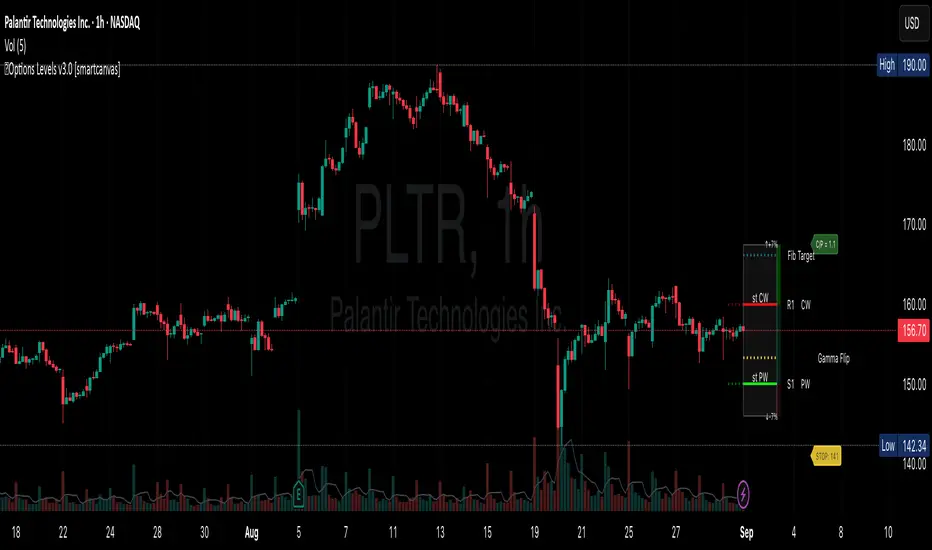
Support and Resistance levels from Options DataINTRODUCTION
This script is designed to visualize key support and resistance levels derived from options data on TradingView charts. It overlays lines, labels, and boxes to highlight levels such as Put Walls (gamma support), Call Walls (gamma resistance), Gamma Flip points, Vanna levels, and more.
These levels are intended to help traders identify potential areas of price magnetism, reversal, or breakout based on options market dynamics. All calculations and visualizations are based on user-provided data pasted into the input field, as Pine Script cannot directly fetch external options data due to platform limitations (explained below).
For convenience, my website allows users to interact with a bot that will generate the string for up to 30 tickers at once getting nearly real-time data on demand (data is cached for 15min). With the output string pasted into this indicator, it's a bliss to shuffle through your portfolio and see those levels for each ticker.
The script is open-source under TradingView's terms, allowing users to study, modify, and improve it. It draws inspiration from common options-derived metrics like gamma exposure and vanna, which are widely discussed in financial literature. No external code is copied without rights; all logic is original or based on standard mathematical formulas.
How the Options Levels Are Calculated
The levels displayed by this script are not computed within Pine Script itself—instead, they rely on pre-calculated values provided by the user (via a pasted data string). These values are derived from options chain data fetched from financial APIs (e.g., using libraries like yfinance in Python). Here's a step-by-step overview of how these levels are generally calculated externally before being input into the script:
Fetching Options Data:
Historical and current options chain data for a ticker (e.g., strikes, open interest, volume, implied volatility, expirations) is retrieved for near-term expirations (e.g., up to 90 days).
Current stock price is obtained from recent history.
Gamma Support (Put Wall) and Resistance (Call Wall):
Gamma Calculation: For each option, gamma (the rate of change of delta) is computed using the Black-Scholes formula:
gamma = N'(d1) / (S * sigma * sqrt(T))
where S is the stock price, K is the strike, T is time to expiration (in years), sigma is implied volatility, r is the risk-free rate (e.g., 0.0445), and N'(d1) is the normal probability density function.
Weighted gamma is multiplied by open interest and aggregated by strike.
The Put Wall is the strike below the current price with the highest weighted gamma from puts (acting as support).
The Call Wall is the strike above the current price with the highest weighted gamma from calls (acting as resistance).
Short-term versions focus on strikes closer to the money (e.g., within 10-15% of the price).
Gamma Flip Level:
Net dealer gamma exposure (GEX) is calculated across all strikes:
GEX = sum (gamma * OI * 100 * S^2 * sign * decay)
where sign is +1 for calls/-1 for puts, and decay is 1 / sqrt(T).
The flip point is the price where net GEX changes sign (from positive to negative or vice versa), interpolated between strikes.
Vanna Levels:
Vanna (sensitivity of delta to volatility) is calculated:
vanna = -N'(d1) * d2 / sigma
where d2 = d1 - sigma * sqrt(T).
Weighted by open interest, the highest positive and negative vanna strikes are identified.
Other Levels:
S1/R1: Significant strikes with high combined open interest and volume (80% OI + 20% volume), below/above price for support/resistance.
Implied Move: ATM implied volatility scaled by S * sigma * sqrt(d/365) (e.g., for 7 days).
Call/Put Ratio: Total call contracts divided by put contracts (OI + volume).
IV Percentage: Average ATM implied volatility.
Options Activity Level: Average contracts per unique strike, binned into levels (0-4).
Stop Loss: Dynamically set below the lowest support (e.g., Put Wall, Gamma Flip), adjusted by IV (tighter in low IV).
Fib Target: 1.618 extension from Put Wall to Call Wall range.
Previous day levels are stored for comparison (e.g., to detect Call Wall movement >2.5% for alerts).
Effect as Support and Resistance in Technical Trading
Options levels like gamma walls influence price action due to market maker hedging:
Put Wall (Gamma Support): High put gamma below price creates a "magnet" effect—market makers buy stock as price falls, providing support. Traders might look for bounces here as entry points for longs.
Call Wall (Gamma Resistance): High call gamma above price leads to selling pressure from hedging, acting as resistance. Rejections here could signal trims, sells or even shorts.
Gamma Flip: Where gamma exposure flips sign, often a volatility pivot—crossing it can accelerate moves (bullish above, bearish below).
Vanna Levels: Positive/negative vanna indicate volatility sensitivity; crosses may signal regime shifts.
Implied Move: Shows expected range; prices outside suggest overextension.
S1/R1 and Fib Target: Volume/OI clusters act as classic S/R; Fib extensions project upside targets post-breakout.
In trading, these are not guarantees—combine with TA (e.g., volume, trends). High activity levels imply stronger effects; low CP ratio suggests bearish sentiment. Alerts trigger on proximities/crosses for awareness, not advice.
Limitations of the TradingView Platform for Data Pulling
TradingView's Pine Script is sandboxed for security and performance:
No direct internet access or API calls (e.g., can't fetch yfinance data in-script).
Limited to chart data/symbol info; no real-time options chains.
Inputs are static per load; updates require manual pasting.
Caching isn't persistent across sessions.
This prevents dynamic data pulling, ensuring scripts remain lightweight but requiring external tools for fresh data.
Creative Solution for On-Demand Data Pulling
To overcome these limitations, users can use external tools or scripts (e.g., Python-based) to fetch and compute levels on demand. The tool processes tickers, generates a formatted string (e.g., "TICKER:level1,level2,...;TIMESTAMP:unix;"), and users paste it into the script's input. This keeps data fresh without violating platform rules, as computation happens off-platform. For example, run a local script to query APIs and output the string—adaptable for any ticker.
Script Functionality Breakdown
Inputs: Custom data string (parsed for levels/timestamp); toggles for short-term/previous/Vanna/stop loss; style options (colors, transparency).
Parsing: Extracts levels for the chart symbol; gets timestamp for "updated ago" display.
Drawing: Lines/labels for levels; boxes for gamma zones/implied move; clears old elements on updates.
Info Panel: Top-right summary with metrics (CP ratio, IV, distances, activity); emojis for quick status.
Alerts: Conditions for proximities, crosses, bounces (e.g., 0.5% bounce from Put Wall).
Performance: Uses vars for persistence; efficient for real-time.
This script is educational—test thoroughly. Not financial advice; past performance isn't indicative of future results. Feedback welcome via TradingView comments.
BTC/USD 3分バイナリー予測【完全修正版v7.2】## BTC/USD 3-Minute Binary Prediction Indicator v7.2 Documentation
### Overview
This indicator predicts whether BTCUSD price will move ±$25 or more within 3 minutes using a 5-layer filter system and pattern recognition. Designed for 30-second timeframe analysis with statistical tracking.
### ⚠️ Critical Warnings
- **This is a prediction tool, NOT a profit guarantee**
- **30-second timeframe ONLY** (Will not function correctly on other timeframes)
- **BTCUSD pair ONLY**
- **Past performance does not guarantee future results**
- **Test thoroughly in demo before live trading**
- **You can lose your entire investment**
### Core Components
#### 1. Five-Layer Filter System
```
Layer 1: Trend Alignment (25 points) - EMA configuration analysis
Layer 2: Indicator Confluence (25 points) - RSI + MACD confirmation
Layer 3: Volume Analysis (20 points) - Abnormal volume detection
Layer 4: Key Levels (15 points) - Support/Resistance proximity
Layer 5: Momentum (15 points) - Price acceleration measurement
```
#### 2. Pattern Recognition Engine
- Double Top/Bottom formations
- Triangle patterns (Symmetrical, Ascending, Descending)
- Channel patterns
- Candlestick patterns (Engulfing, Hammer, Hanging Man)
#### 3. Performance Tracking
- Overall win rate
- Hourly performance
- Daily performance
- Real-time statistics
### Input Parameters
#### Basic Settings
- `Range Width ($)`: Target price movement (Default: $50 = ±$25)
- `Minimum Confidence (%)`: Required confidence for entry (Default: 75%)
- `Max Daily Trades`: Overtrading prevention (Default: 5)
#### Filter Settings
- `Trend Filter`: EMA alignment validation
- `Volume Confirmation`: Volume spike detection
- `S/R Filter`: Key level analysis
- `Momentum Alignment`: Directional strength confirmation
#### Display Settings
- `Minimal Mode`: Reduced visual elements for experienced users
- `Pattern Display`: Visual pattern overlays
- `EMA Lines`: Moving average visualization
### Usage Instructions
#### Setup Process
1. Open BTCUSD chart on TradingView
2. **Set timeframe to 30 seconds** (CRITICAL)
3. Add indicator to chart
4. Adjust parameters if needed
#### Reading Signals
**Decision Panel (Left Side)**
- `HIGH`: Predicts +$25 move in 3 minutes
- `LOW`: Predicts -$25 move in 3 minutes
- `WAIT`: Conditions building, no entry yet
- `STAY`: No trade opportunity
**F-Score Interpretation**
- 65+ points: Direction suggestion (light color)
- 80+ points: Strong signal (solid color)
- Entry ready: Exclamation mark (!)
**Statistics Panel (Right Side)**
- Win rate: Percentage of successful predictions
- 1H Stats: Last hour performance
- Daily Stats: Today's results
#### Entry Execution
1. Wait for `HIGH!` or `LOW!` in decision panel
2. Large arrow appears on chart (▲ for HIGH, ▼ for LOW)
3. Enter at **next candle open**
4. Result evaluated after 3 minutes (6 candles)
### Algorithm Logic
#### Early Entry System (v7.2 Feature)
The indicator uses predictive analysis starting at F-Score 65 instead of waiting for 80:
- Faster signal generation
- Reduced opportunity loss
- Slightly lower win rate trade-off
#### Confidence Calculation
```
Base confidence: 50%
+ Filter score bonus
+ Pattern recognition bonus
+ Volatility adjustment
- Risk factors
= Final confidence (50-95%)
```
### Technical Specifications
#### Multi-Timeframe Analysis
- Primary: 30-second chart
- Secondary: 1-minute data
- Reference: 5-minute trend
#### Data Processing
- Real-time tick analysis
- No repainting (signals are final)
- Historical verification system
### Limitations & Known Issues
1. **Spread/Commission Not Included**: Actual profits will be lower
2. **30-Second Noise**: High false signal risk on ultra-short timeframe
3. **Network Latency**: Execution delays not accounted for
4. **Market Conditions**: Performance varies with volatility
5. **Algorithm Trading**: Cannot compete with HFT systems
### Performance Metrics
- Target Win Rate: 83% (aspirational)
- Evaluation Period: 3 minutes
- Risk per trade: Fixed ±$25
- Maximum daily exposure: 5 trades
### Troubleshooting Guide
**No signals appearing?**
- Check F-Score (needs 65+)
- Verify 30-second timeframe
- Ensure BTCUSD pair selected
**Low win rate?**
- Only trade 75%+ confidence signals
- Respect daily trade limit
- Avoid news events
**Pattern shows "-"?**
- Normal when no clear pattern exists
- Not all market conditions produce patterns
### Code Modification Notes
Written in Pine Script v6. Key considerations for modifications:
- Global variables use `var` for persistence
- Drawing objects require manual management
- Bar counting varies by timeframe
- Pattern detection runs on confirmed bars only
### Risk Disclosure
**IMPORTANT**: Trading cryptocurrencies involves substantial risk of loss and is not suitable for all investors. The high degree of leverage can work against you as well as for you. Before deciding to trade, you should carefully consider your investment objectives, level of experience, and risk appetite. The possibility exists that you could sustain a loss of some or all of your initial investment and therefore you should not invest money that you cannot afford to lose.
### Support & Updates
- Report issues in TradingView comments
- Check for updates regularly
- Version 7.2 is current release
- Community feedback welcome
### Legal Notice
This indicator is provided for educational and research purposes only. It should not be construed as investment advice. The authors and distributors of this indicator accept no liability for losses incurred through its use. Always consult with a qualified financial advisor before making investment decisions.
---
*Version: 7.2*
*License: Mozilla Public License 2.0*
*Author: *
*Last Updated: 2024*
**FINAL WARNING: This indicator cannot predict the future. Use at your own risk. Start with demo trading. Never trade with money you cannot afford to lose.**

Pivot Points. High & Lows By Reversal PercentageLibrary "Pivot Points. High & Lows By Reversal Percentage" by Jal9000
This Pine Script library provides a robust function for identifying and tracking pivot points (reversal points) in price data, suitable for integration into custom trading indicators and strategies.
🛠️ Main Features:
- ✅ Identifies pivot highs and lows based on configurable price movement thresholds.
- ✅ Lightweight. No candle backtracing used. Much less computation heavy.
- ✅ Supports multiple calls (with different values) within a single script.
- ✅ Compatible with request.security for multi-timeframe analysis.
- ✅ Returns both confirmed and temporary pivots for flexible integration.
- ✅ Pinescript V5 and V6 compliant code.
Purpose:
The pivots library enables Pine Script developers to easily add pivot point detection to their scripts. It identifies significant price reversals by evaluating price movements against a minimum range threshold ( min_range_pct ) and confirming reversals based on a percentage ( reversal_pct ) of the prior trend’s magnitude. The library supports multiple simultaneous calls with different settings, making it ideal for multi-timeframe strategies.
How It Works:
The library’s f_calculatePivot function tracks price movements to detect pivot points:
Minimum Range Threshold : A potential pivot is considered if the price moves beyond the min_range_pct percentage of the current high (for a high pivot) or low (for a low pivot), ensuring sufficient movement.
Reversal Confirmation : A pivot is confirmed if the price reverses from the potential pivot by at least the reversal_pct percentage of the distance between the last confirmed pivot and the current potential pivot, measuring the retracement relative to the prior trend’s magnitude.
The function alternates between tracking highs (in an uptrend) and lows (in a downtrend), updating the trend when a pivot is confirmed.
State management uses an array of pivot_state objects, allowing independent calculations for different timeframes and min_range_pct values within the same script.
## Technical Reference
Functions:
f_calculatePivot(series float _high, series float _low, float _min_range_pct, float _reversal_pct) →
- Parameters:
_high : The high price series (e.g., high or math.max(open, close) ).
_low : The low price series (e.g., low or math.min(open, close) ).
_min_range_pct : The minimum percentage price movement to consider a potential pivot.
_reversal_pct : The percentage of the prior trend’s distance required to confirm a pivot.
- Returns:
A tuple containing:
isNewPivot : Boolean indicating if a new pivot was confirmed.
last_confirmed_pivot : The most recent confirmed pivot (type pivot ).
temp_pivot : The current temporary pivot (type pivot ).
Pivot type:
idx (series int) : Bar index of the pivot.
typ (series int) : Type of pivot ( PIVOT_HIGH or PIVOT_LOW ).
prc (series float) : Price of the pivot.
tme (series int) : Timestamp of the pivot.
Constants (internal):
TREND_LONG , TREND_SHORT : Trend direction indicators (1, -1).
PIVOT_HIGH , PIVOT_LOW : Pivot type indicators (1, -1).
✨ Example of Use:
//@version=5
indicator("Pivot Example", overlay=true)
import jal9000/pivots/1 as pivots
// Inputs
min_range_pct = input.float(20.0, 'Min Range %')
reversal_pct = input.float(30.0, 'Reversal %')
ignore_wick = input.bool(true, 'Ignore wick')
h = ignore_wick ? math.max(open, close) : high
l = ignore_wick ? math.min(open, close) : low
// Call the function with high, low, and input parameters
= pivots.f_calculatePivot(h, l, min_range_pct, reversal_pct)
// Variable to store previous confirmed pivot outside the function
var pivots.pivot prev_confirmed_pivot = na
// Draw the line if a new pivot is confirmed and previous pivot exists
if is_new_pivot
if not na(prev_confirmed_pivot) and not na(new_confirmed_pivot)
line.new(x1 = prev_confirmed_pivot.idx, y1 = prev_confirmed_pivot.prc, x2 = new_confirmed_pivot.idx, y2 = new_confirmed_pivot.prc, color = color.blue, width = 1)
prev_confirmed_pivot := new_confirmed_pivot
## Release Notes
v1
- Initial release of the pivots library with f_calculatePivot function for detecting pivot points and supporting multiple configurations and timeframes.
v2
- Code is Pinescript V6 ready. Remains identified as V5, but changing the version number is the only thing that is required to be v6.
Trapped Traders [ScorsoneEnterprises]This indicator identifies and visualizes trapped traders - market participants caught on the wrong side of price movements with significant volume imbalances. By analyzing volume delta at specific price levels, it reveals where traders are likely experiencing unrealized losses and may be forced to exit their positions.
The point of this tool is to identify where the liquidity in a trend may be.
var lowerTimeframe = switch
useCustomTimeframeInput => lowerTimeframeInput
timeframe.isseconds => "1S"
timeframe.isintraday => "1"
timeframe.isdaily => "5"
=> "60"
= ta.requestVolumeDelta(lowerTimeframe)
price_quantity = map.new()
is_red_candle = close < open
is_green_candle = close > open
for i=0 to lkb-1 by 1
current_vol = price_quantity.get(close)
new_vol = na(current_vol) ? lastVolume : current_vol + lastVolume
price_quantity.put(close, new_vol)
if is_green_candle and new_vol < 0
price_quantity.put(close, new_vol)
else if is_red_candle and new_vol > 0
price_quantity.put(close, new_vol)
We see in this snippet, the lastVolume variable is the most recent volume delta we can receive from the lower timeframe, we keep updating the price level we're keeping track of with that lastVolume from the lower timeframe.
This is the bulk of the concept as this level and size gives us the idea of how many traders were on the wrong side of the trend, and acting as liquidity for the profitable entries. The more, the stronger.
There are 3 ways to visualize this. A basic label, that will display the size and if positive or negative next to the bar, a gradient line that goes 10 bars to the future to be used as a support or resistance line that includes the quantity, and a bubble chart with the quantity. The larger the quantity, the bigger the bubble.
We see in this example on NYMEX:CL1! that there are lines plotted throughout this price action that price interacts with in meaningful way. There are consistently many levels for us.
Here on CME_MINI:ES1! we see the labels on the chart, and the size set to large. It is the same concept just another way to view it.
This chart of CME_MINI:RTY1! shows the bubble chart visualization. It is a way to view it that is pretty non invasive on the chart.
Every timeframe is supported including daily, weekly, and monthly.
The included settings are the display style, like mentioned above. If the user would like to see the volume numbers on the chart. The text size along with the transparency percentage. Following that is the settings for which lower timeframe to calculate the volume delta on. Finally, if you would like to see your inputs in the status line.
No indicator is 100% accurate, use "Trapped Traders" along with your own discretion.

Markov Chain [3D] | FractalystWhat exactly is a Markov Chain?
This indicator uses a Markov Chain model to analyze, quantify, and visualize the transitions between market regimes (Bull, Bear, Neutral) on your chart. It dynamically detects these regimes in real-time, calculates transition probabilities, and displays them as animated 3D spheres and arrows, giving traders intuitive insight into current and future market conditions.
How does a Markov Chain work, and how should I read this spheres-and-arrows diagram?
Think of three weather modes: Sunny, Rainy, Cloudy.
Each sphere is one mode. The loop on a sphere means “stay the same next step” (e.g., Sunny again tomorrow).
The arrows leaving a sphere show where things usually go next if they change (e.g., Sunny moving to Cloudy).
Some paths matter more than others. A more prominent loop means the current mode tends to persist. A more prominent outgoing arrow means a change to that destination is the usual next step.
Direction isn’t symmetric: moving Sunny→Cloudy can behave differently than Cloudy→Sunny.
Now relabel the spheres to markets: Bull, Bear, Neutral.
Spheres: market regimes (uptrend, downtrend, range).
Self‑loop: tendency for the current regime to continue on the next bar.
Arrows: the most common next regime if a switch happens.
How to read: Start at the sphere that matches current bar state. If the loop stands out, expect continuation. If one outgoing path stands out, that switch is the typical next step. Opposite directions can differ (Bear→Neutral doesn’t have to match Neutral→Bear).
What states and transitions are shown?
The three market states visualized are:
Bullish (Bull): Upward or strong-market regime.
Bearish (Bear): Downward or weak-market regime.
Neutral: Sideways or range-bound regime.
Bidirectional animated arrows and probability labels show how likely the market is to move from one regime to another (e.g., Bull → Bear or Neutral → Bull).
How does the regime detection system work?
You can use either built-in price returns (based on adaptive Z-score normalization) or supply three custom indicators (such as volume, oscillators, etc.).
Values are statistically normalized (Z-scored) over a configurable lookback period.
The normalized outputs are classified into Bull, Bear, or Neutral zones.
If using three indicators, their regime signals are averaged and smoothed for robustness.
How are transition probabilities calculated?
On every confirmed bar, the algorithm tracks the sequence of detected market states, then builds a rolling window of transitions.
The code maintains a transition count matrix for all regime pairs (e.g., Bull → Bear).
Transition probabilities are extracted for each possible state change using Laplace smoothing for numerical stability, and frequently updated in real-time.
What is unique about the visualization?
3D animated spheres represent each regime and change visually when active.
Animated, bidirectional arrows reveal transition probabilities and allow you to see both dominant and less likely regime flows.
Particles (moving dots) animate along the arrows, enhancing the perception of regime flow direction and speed.
All elements dynamically update with each new price bar, providing a live market map in an intuitive, engaging format.
Can I use custom indicators for regime classification?
Yes! Enable the "Custom Indicators" switch and select any three chart series as inputs. These will be normalized and combined (each with equal weight), broadening the regime classification beyond just price-based movement.
What does the “Lookback Period” control?
Lookback Period (default: 100) sets how much historical data builds the probability matrix. Shorter periods adapt faster to regime changes but may be noisier. Longer periods are more stable but slower to adapt.
How is this different from a Hidden Markov Model (HMM)?
It sets the window for both regime detection and probability calculations. Lower values make the system more reactive, but potentially noisier. Higher values smooth estimates and make the system more robust.
How is this Markov Chain different from a Hidden Markov Model (HMM)?
Markov Chain (as here): All market regimes (Bull, Bear, Neutral) are directly observable on the chart. The transition matrix is built from actual detected regimes, keeping the model simple and interpretable.
Hidden Markov Model: The actual regimes are unobservable ("hidden") and must be inferred from market output or indicator "emissions" using statistical learning algorithms. HMMs are more complex, can capture more subtle structure, but are harder to visualize and require additional machine learning steps for training.
A standard Markov Chain models transitions between observable states using a simple transition matrix, while a Hidden Markov Model assumes the true states are hidden (latent) and must be inferred from observable “emissions” like price or volume data. In practical terms, a Markov Chain is transparent and easier to implement and interpret; an HMM is more expressive but requires statistical inference to estimate hidden states from data.
Markov Chain: states are observable; you directly count or estimate transition probabilities between visible states. This makes it simpler, faster, and easier to validate and tune.
HMM: states are hidden; you only observe emissions generated by those latent states. Learning involves machine learning/statistical algorithms (commonly Baum–Welch/EM for training and Viterbi for decoding) to infer both the transition dynamics and the most likely hidden state sequence from data.
How does the indicator avoid “repainting” or look-ahead bias?
All regime changes and matrix updates happen only on confirmed (closed) bars, so no future data is leaked, ensuring reliable real-time operation.
Are there practical tuning tips?
Tune the Lookback Period for your asset/timeframe: shorter for fast markets, longer for stability.
Use custom indicators if your asset has unique regime drivers.
Watch for rapid changes in transition probabilities as early warning of a possible regime shift.
Who is this indicator for?
Quants and quantitative researchers exploring probabilistic market modeling, especially those interested in regime-switching dynamics and Markov models.
Programmers and system developers who need a probabilistic regime filter for systematic and algorithmic backtesting:
The Markov Chain indicator is ideally suited for programmatic integration via its bias output (1 = Bull, 0 = Neutral, -1 = Bear).
Although the visualization is engaging, the core output is designed for automated, rules-based workflows—not for discretionary/manual trading decisions.
Developers can connect the indicator’s output directly to their Pine Script logic (using input.source()), allowing rapid and robust backtesting of regime-based strategies.
It acts as a plug-and-play regime filter: simply plug the bias output into your entry/exit logic, and you have a scientifically robust, probabilistically-derived signal for filtering, timing, position sizing, or risk regimes.
The MC's output is intentionally "trinary" (1/0/-1), focusing on clear regime states for unambiguous decision-making in code. If you require nuanced, multi-probability or soft-label state vectors, consider expanding the indicator or stacking it with a probability-weighted logic layer in your scripting.
Because it avoids subjectivity, this approach is optimal for systematic quants, algo developers building backtested, repeatable strategies based on probabilistic regime analysis.
What's the mathematical foundation behind this?
The mathematical foundation behind this Markov Chain indicator—and probabilistic regime detection in finance—draws from two principal models: the (standard) Markov Chain and the Hidden Markov Model (HMM).
How to use this indicator programmatically?
The Markov Chain indicator automatically exports a bias value (+1 for Bullish, -1 for Bearish, 0 for Neutral) as a plot visible in the Data Window. This allows you to integrate its regime signal into your own scripts and strategies for backtesting, automation, or live trading.
Step-by-Step Integration with Pine Script (input.source)
Add the Markov Chain indicator to your chart.
This must be done first, since your custom script will "pull" the bias signal from the indicator's plot.
In your strategy, create an input using input.source()
Example:
//@version=5
strategy("MC Bias Strategy Example")
mcBias = input.source(close, "MC Bias Source")
After saving, go to your script’s settings. For the “MC Bias Source” input, select the plot/output of the Markov Chain indicator (typically its bias plot).
Use the bias in your trading logic
Example (long only on Bull, flat otherwise):
if mcBias == 1
strategy.entry("Long", strategy.long)
else
strategy.close("Long")
For more advanced workflows, combine mcBias with additional filters or trailing stops.
How does this work behind-the-scenes?
TradingView’s input.source() lets you use any plot from another indicator as a real-time, “live” data feed in your own script (source).
The selected bias signal is available to your Pine code as a variable, enabling logical decisions based on regime (trend-following, mean-reversion, etc.).
This enables powerful strategy modularity : decouple regime detection from entry/exit logic, allowing fast experimentation without rewriting core signal code.
Integrating 45+ Indicators with Your Markov Chain — How & Why
The Enhanced Custom Indicators Export script exports a massive suite of over 45 technical indicators—ranging from classic momentum (RSI, MACD, Stochastic, etc.) to trend, volume, volatility, and oscillator tools—all pre-calculated, centered/scaled, and available as plots.
// Enhanced Custom Indicators Export - 45 Technical Indicators
// Comprehensive technical analysis suite for advanced market regime detection
//@version=6
indicator('Enhanced Custom Indicators Export | Fractalyst', shorttitle='Enhanced CI Export', overlay=false, scale=scale.right, max_labels_count=500, max_lines_count=500)
// |----- Input Parameters -----| //
momentum_group = "Momentum Indicators"
trend_group = "Trend Indicators"
volume_group = "Volume Indicators"
volatility_group = "Volatility Indicators"
oscillator_group = "Oscillator Indicators"
display_group = "Display Settings"
// Common lengths
length_14 = input.int(14, "Standard Length (14)", minval=1, maxval=100, group=momentum_group)
length_20 = input.int(20, "Medium Length (20)", minval=1, maxval=200, group=trend_group)
length_50 = input.int(50, "Long Length (50)", minval=1, maxval=200, group=trend_group)
// Display options
show_table = input.bool(true, "Show Values Table", group=display_group)
table_size = input.string("Small", "Table Size", options= , group=display_group)
// |----- MOMENTUM INDICATORS (15 indicators) -----| //
// 1. RSI (Relative Strength Index)
rsi_14 = ta.rsi(close, length_14)
rsi_centered = rsi_14 - 50
// 2. Stochastic Oscillator
stoch_k = ta.stoch(close, high, low, length_14)
stoch_d = ta.sma(stoch_k, 3)
stoch_centered = stoch_k - 50
// 3. Williams %R
williams_r = ta.stoch(close, high, low, length_14) - 100
// 4. MACD (Moving Average Convergence Divergence)
= ta.macd(close, 12, 26, 9)
// 5. Momentum (Rate of Change)
momentum = ta.mom(close, length_14)
momentum_pct = (momentum / close ) * 100
// 6. Rate of Change (ROC)
roc = ta.roc(close, length_14)
// 7. Commodity Channel Index (CCI)
cci = ta.cci(close, length_20)
// 8. Money Flow Index (MFI)
mfi = ta.mfi(close, length_14)
mfi_centered = mfi - 50
// 9. Awesome Oscillator (AO)
ao = ta.sma(hl2, 5) - ta.sma(hl2, 34)
// 10. Accelerator Oscillator (AC)
ac = ao - ta.sma(ao, 5)
// 11. Chande Momentum Oscillator (CMO)
cmo = ta.cmo(close, length_14)
// 12. Detrended Price Oscillator (DPO)
dpo = close - ta.sma(close, length_20)
// 13. Price Oscillator (PPO)
ppo = ta.sma(close, 12) - ta.sma(close, 26)
ppo_pct = (ppo / ta.sma(close, 26)) * 100
// 14. TRIX
trix_ema1 = ta.ema(close, length_14)
trix_ema2 = ta.ema(trix_ema1, length_14)
trix_ema3 = ta.ema(trix_ema2, length_14)
trix = ta.roc(trix_ema3, 1) * 10000
// 15. Klinger Oscillator
klinger = ta.ema(volume * (high + low + close) / 3, 34) - ta.ema(volume * (high + low + close) / 3, 55)
// 16. Fisher Transform
fisher_hl2 = 0.5 * (hl2 - ta.lowest(hl2, 10)) / (ta.highest(hl2, 10) - ta.lowest(hl2, 10)) - 0.25
fisher = 0.5 * math.log((1 + fisher_hl2) / (1 - fisher_hl2))
// 17. Stochastic RSI
stoch_rsi = ta.stoch(rsi_14, rsi_14, rsi_14, length_14)
stoch_rsi_centered = stoch_rsi - 50
// 18. Relative Vigor Index (RVI)
rvi_num = ta.swma(close - open)
rvi_den = ta.swma(high - low)
rvi = rvi_den != 0 ? rvi_num / rvi_den : 0
// 19. Balance of Power (BOP)
bop = (close - open) / (high - low)
// |----- TREND INDICATORS (10 indicators) -----| //
// 20. Simple Moving Average Momentum
sma_20 = ta.sma(close, length_20)
sma_momentum = ((close - sma_20) / sma_20) * 100
// 21. Exponential Moving Average Momentum
ema_20 = ta.ema(close, length_20)
ema_momentum = ((close - ema_20) / ema_20) * 100
// 22. Parabolic SAR
sar = ta.sar(0.02, 0.02, 0.2)
sar_trend = close > sar ? 1 : -1
// 23. Linear Regression Slope
lr_slope = ta.linreg(close, length_20, 0) - ta.linreg(close, length_20, 1)
// 24. Moving Average Convergence (MAC)
mac = ta.sma(close, 10) - ta.sma(close, 30)
// 25. Trend Intensity Index (TII)
tii_sum = 0.0
for i = 1 to length_20
tii_sum += close > close ? 1 : 0
tii = (tii_sum / length_20) * 100
// 26. Ichimoku Cloud Components
ichimoku_tenkan = (ta.highest(high, 9) + ta.lowest(low, 9)) / 2
ichimoku_kijun = (ta.highest(high, 26) + ta.lowest(low, 26)) / 2
ichimoku_signal = ichimoku_tenkan > ichimoku_kijun ? 1 : -1
// 27. MESA Adaptive Moving Average (MAMA)
mama_alpha = 2.0 / (length_20 + 1)
mama = ta.ema(close, length_20)
mama_momentum = ((close - mama) / mama) * 100
// 28. Zero Lag Exponential Moving Average (ZLEMA)
zlema_lag = math.round((length_20 - 1) / 2)
zlema_data = close + (close - close )
zlema = ta.ema(zlema_data, length_20)
zlema_momentum = ((close - zlema) / zlema) * 100
// |----- VOLUME INDICATORS (6 indicators) -----| //
// 29. On-Balance Volume (OBV)
obv = ta.obv
// 30. Volume Rate of Change (VROC)
vroc = ta.roc(volume, length_14)
// 31. Price Volume Trend (PVT)
pvt = ta.pvt
// 32. Negative Volume Index (NVI)
nvi = 0.0
nvi := volume < volume ? nvi + ((close - close ) / close ) * nvi : nvi
// 33. Positive Volume Index (PVI)
pvi = 0.0
pvi := volume > volume ? pvi + ((close - close ) / close ) * pvi : pvi
// 34. Volume Oscillator
vol_osc = ta.sma(volume, 5) - ta.sma(volume, 10)
// 35. Ease of Movement (EOM)
eom_distance = high - low
eom_box_height = volume / 1000000
eom = eom_box_height != 0 ? eom_distance / eom_box_height : 0
eom_sma = ta.sma(eom, length_14)
// 36. Force Index
force_index = volume * (close - close )
force_index_sma = ta.sma(force_index, length_14)
// |----- VOLATILITY INDICATORS (10 indicators) -----| //
// 37. Average True Range (ATR)
atr = ta.atr(length_14)
atr_pct = (atr / close) * 100
// 38. Bollinger Bands Position
bb_basis = ta.sma(close, length_20)
bb_dev = 2.0 * ta.stdev(close, length_20)
bb_upper = bb_basis + bb_dev
bb_lower = bb_basis - bb_dev
bb_position = bb_dev != 0 ? (close - bb_basis) / bb_dev : 0
bb_width = bb_dev != 0 ? (bb_upper - bb_lower) / bb_basis * 100 : 0
// 39. Keltner Channels Position
kc_basis = ta.ema(close, length_20)
kc_range = ta.ema(ta.tr, length_20)
kc_upper = kc_basis + (2.0 * kc_range)
kc_lower = kc_basis - (2.0 * kc_range)
kc_position = kc_range != 0 ? (close - kc_basis) / kc_range : 0
// 40. Donchian Channels Position
dc_upper = ta.highest(high, length_20)
dc_lower = ta.lowest(low, length_20)
dc_basis = (dc_upper + dc_lower) / 2
dc_position = (dc_upper - dc_lower) != 0 ? (close - dc_basis) / (dc_upper - dc_lower) : 0
// 41. Standard Deviation
std_dev = ta.stdev(close, length_20)
std_dev_pct = (std_dev / close) * 100
// 42. Relative Volatility Index (RVI)
rvi_up = ta.stdev(close > close ? close : 0, length_14)
rvi_down = ta.stdev(close < close ? close : 0, length_14)
rvi_total = rvi_up + rvi_down
rvi_volatility = rvi_total != 0 ? (rvi_up / rvi_total) * 100 : 50
// 43. Historical Volatility
hv_returns = math.log(close / close )
hv = ta.stdev(hv_returns, length_20) * math.sqrt(252) * 100
// 44. Garman-Klass Volatility
gk_vol = math.log(high/low) * math.log(high/low) - (2*math.log(2)-1) * math.log(close/open) * math.log(close/open)
gk_volatility = math.sqrt(ta.sma(gk_vol, length_20)) * 100
// 45. Parkinson Volatility
park_vol = math.log(high/low) * math.log(high/low)
parkinson = math.sqrt(ta.sma(park_vol, length_20) / (4 * math.log(2))) * 100
// 46. Rogers-Satchell Volatility
rs_vol = math.log(high/close) * math.log(high/open) + math.log(low/close) * math.log(low/open)
rogers_satchell = math.sqrt(ta.sma(rs_vol, length_20)) * 100
// |----- OSCILLATOR INDICATORS (5 indicators) -----| //
// 47. Elder Ray Index
elder_bull = high - ta.ema(close, 13)
elder_bear = low - ta.ema(close, 13)
elder_power = elder_bull + elder_bear
// 48. Schaff Trend Cycle (STC)
stc_macd = ta.ema(close, 23) - ta.ema(close, 50)
stc_k = ta.stoch(stc_macd, stc_macd, stc_macd, 10)
stc_d = ta.ema(stc_k, 3)
stc = ta.stoch(stc_d, stc_d, stc_d, 10)
// 49. Coppock Curve
coppock_roc1 = ta.roc(close, 14)
coppock_roc2 = ta.roc(close, 11)
coppock = ta.wma(coppock_roc1 + coppock_roc2, 10)
// 50. Know Sure Thing (KST)
kst_roc1 = ta.roc(close, 10)
kst_roc2 = ta.roc(close, 15)
kst_roc3 = ta.roc(close, 20)
kst_roc4 = ta.roc(close, 30)
kst = ta.sma(kst_roc1, 10) + 2*ta.sma(kst_roc2, 10) + 3*ta.sma(kst_roc3, 10) + 4*ta.sma(kst_roc4, 15)
// 51. Percentage Price Oscillator (PPO)
ppo_line = ((ta.ema(close, 12) - ta.ema(close, 26)) / ta.ema(close, 26)) * 100
ppo_signal = ta.ema(ppo_line, 9)
ppo_histogram = ppo_line - ppo_signal
// |----- PLOT MAIN INDICATORS -----| //
// Plot key momentum indicators
plot(rsi_centered, title="01_RSI_Centered", color=color.purple, linewidth=1)
plot(stoch_centered, title="02_Stoch_Centered", color=color.blue, linewidth=1)
plot(williams_r, title="03_Williams_R", color=color.red, linewidth=1)
plot(macd_histogram, title="04_MACD_Histogram", color=color.orange, linewidth=1)
plot(cci, title="05_CCI", color=color.green, linewidth=1)
// Plot trend indicators
plot(sma_momentum, title="06_SMA_Momentum", color=color.navy, linewidth=1)
plot(ema_momentum, title="07_EMA_Momentum", color=color.maroon, linewidth=1)
plot(sar_trend, title="08_SAR_Trend", color=color.teal, linewidth=1)
plot(lr_slope, title="09_LR_Slope", color=color.lime, linewidth=1)
plot(mac, title="10_MAC", color=color.fuchsia, linewidth=1)
// Plot volatility indicators
plot(atr_pct, title="11_ATR_Pct", color=color.yellow, linewidth=1)
plot(bb_position, title="12_BB_Position", color=color.aqua, linewidth=1)
plot(kc_position, title="13_KC_Position", color=color.olive, linewidth=1)
plot(std_dev_pct, title="14_StdDev_Pct", color=color.silver, linewidth=1)
plot(bb_width, title="15_BB_Width", color=color.gray, linewidth=1)
// Plot volume indicators
plot(vroc, title="16_VROC", color=color.blue, linewidth=1)
plot(eom_sma, title="17_EOM", color=color.red, linewidth=1)
plot(vol_osc, title="18_Vol_Osc", color=color.green, linewidth=1)
plot(force_index_sma, title="19_Force_Index", color=color.orange, linewidth=1)
plot(obv, title="20_OBV", color=color.purple, linewidth=1)
// Plot additional oscillators
plot(ao, title="21_Awesome_Osc", color=color.navy, linewidth=1)
plot(cmo, title="22_CMO", color=color.maroon, linewidth=1)
plot(dpo, title="23_DPO", color=color.teal, linewidth=1)
plot(trix, title="24_TRIX", color=color.lime, linewidth=1)
plot(fisher, title="25_Fisher", color=color.fuchsia, linewidth=1)
// Plot more momentum indicators
plot(mfi_centered, title="26_MFI_Centered", color=color.yellow, linewidth=1)
plot(ac, title="27_AC", color=color.aqua, linewidth=1)
plot(ppo_pct, title="28_PPO_Pct", color=color.olive, linewidth=1)
plot(stoch_rsi_centered, title="29_StochRSI_Centered", color=color.silver, linewidth=1)
plot(klinger, title="30_Klinger", color=color.gray, linewidth=1)
// Plot trend continuation
plot(tii, title="31_TII", color=color.blue, linewidth=1)
plot(ichimoku_signal, title="32_Ichimoku_Signal", color=color.red, linewidth=1)
plot(mama_momentum, title="33_MAMA_Momentum", color=color.green, linewidth=1)
plot(zlema_momentum, title="34_ZLEMA_Momentum", color=color.orange, linewidth=1)
plot(bop, title="35_BOP", color=color.purple, linewidth=1)
// Plot volume continuation
plot(nvi, title="36_NVI", color=color.navy, linewidth=1)
plot(pvi, title="37_PVI", color=color.maroon, linewidth=1)
plot(momentum_pct, title="38_Momentum_Pct", color=color.teal, linewidth=1)
plot(roc, title="39_ROC", color=color.lime, linewidth=1)
plot(rvi, title="40_RVI", color=color.fuchsia, linewidth=1)
// Plot volatility continuation
plot(dc_position, title="41_DC_Position", color=color.yellow, linewidth=1)
plot(rvi_volatility, title="42_RVI_Volatility", color=color.aqua, linewidth=1)
plot(hv, title="43_Historical_Vol", color=color.olive, linewidth=1)
plot(gk_volatility, title="44_GK_Volatility", color=color.silver, linewidth=1)
plot(parkinson, title="45_Parkinson_Vol", color=color.gray, linewidth=1)
// Plot final oscillators
plot(rogers_satchell, title="46_RS_Volatility", color=color.blue, linewidth=1)
plot(elder_power, title="47_Elder_Power", color=color.red, linewidth=1)
plot(stc, title="48_STC", color=color.green, linewidth=1)
plot(coppock, title="49_Coppock", color=color.orange, linewidth=1)
plot(kst, title="50_KST", color=color.purple, linewidth=1)
// Plot final indicators
plot(ppo_histogram, title="51_PPO_Histogram", color=color.navy, linewidth=1)
plot(pvt, title="52_PVT", color=color.maroon, linewidth=1)
// |----- Reference Lines -----| //
hline(0, "Zero Line", color=color.gray, linestyle=hline.style_dashed, linewidth=1)
hline(50, "Midline", color=color.gray, linestyle=hline.style_dotted, linewidth=1)
hline(-50, "Lower Midline", color=color.gray, linestyle=hline.style_dotted, linewidth=1)
hline(25, "Upper Threshold", color=color.gray, linestyle=hline.style_dotted, linewidth=1)
hline(-25, "Lower Threshold", color=color.gray, linestyle=hline.style_dotted, linewidth=1)
// |----- Enhanced Information Table -----| //
if show_table and barstate.islast
table_position = position.top_right
table_text_size = table_size == "Tiny" ? size.tiny : table_size == "Small" ? size.small : size.normal
var table info_table = table.new(table_position, 3, 18, bgcolor=color.new(color.white, 85), border_width=1, border_color=color.gray)
// Headers
table.cell(info_table, 0, 0, 'Category', text_color=color.black, text_size=table_text_size, bgcolor=color.new(color.blue, 70))
table.cell(info_table, 1, 0, 'Indicator', text_color=color.black, text_size=table_text_size, bgcolor=color.new(color.blue, 70))
table.cell(info_table, 2, 0, 'Value', text_color=color.black, text_size=table_text_size, bgcolor=color.new(color.blue, 70))
// Key Momentum Indicators
table.cell(info_table, 0, 1, 'MOMENTUM', text_color=color.purple, text_size=table_text_size, bgcolor=color.new(color.purple, 90))
table.cell(info_table, 1, 1, 'RSI Centered', text_color=color.purple, text_size=table_text_size)
table.cell(info_table, 2, 1, str.tostring(rsi_centered, '0.00'), text_color=color.purple, text_size=table_text_size)
table.cell(info_table, 0, 2, '', text_color=color.blue, text_size=table_text_size)
table.cell(info_table, 1, 2, 'Stoch Centered', text_color=color.blue, text_size=table_text_size)
table.cell(info_table, 2, 2, str.tostring(stoch_centered, '0.00'), text_color=color.blue, text_size=table_text_size)
table.cell(info_table, 0, 3, '', text_color=color.red, text_size=table_text_size)
table.cell(info_table, 1, 3, 'Williams %R', text_color=color.red, text_size=table_text_size)
table.cell(info_table, 2, 3, str.tostring(williams_r, '0.00'), text_color=color.red, text_size=table_text_size)
table.cell(info_table, 0, 4, '', text_color=color.orange, text_size=table_text_size)
table.cell(info_table, 1, 4, 'MACD Histogram', text_color=color.orange, text_size=table_text_size)
table.cell(info_table, 2, 4, str.tostring(macd_histogram, '0.000'), text_color=color.orange, text_size=table_text_size)
table.cell(info_table, 0, 5, '', text_color=color.green, text_size=table_text_size)
table.cell(info_table, 1, 5, 'CCI', text_color=color.green, text_size=table_text_size)
table.cell(info_table, 2, 5, str.tostring(cci, '0.00'), text_color=color.green, text_size=table_text_size)
// Key Trend Indicators
table.cell(info_table, 0, 6, 'TREND', text_color=color.navy, text_size=table_text_size, bgcolor=color.new(color.navy, 90))
table.cell(info_table, 1, 6, 'SMA Momentum %', text_color=color.navy, text_size=table_text_size)
table.cell(info_table, 2, 6, str.tostring(sma_momentum, '0.00'), text_color=color.navy, text_size=table_text_size)
table.cell(info_table, 0, 7, '', text_color=color.maroon, text_size=table_text_size)
table.cell(info_table, 1, 7, 'EMA Momentum %', text_color=color.maroon, text_size=table_text_size)
table.cell(info_table, 2, 7, str.tostring(ema_momentum, '0.00'), text_color=color.maroon, text_size=table_text_size)
table.cell(info_table, 0, 8, '', text_color=color.teal, text_size=table_text_size)
table.cell(info_table, 1, 8, 'SAR Trend', text_color=color.teal, text_size=table_text_size)
table.cell(info_table, 2, 8, str.tostring(sar_trend, '0'), text_color=color.teal, text_size=table_text_size)
table.cell(info_table, 0, 9, '', text_color=color.lime, text_size=table_text_size)
table.cell(info_table, 1, 9, 'Linear Regression', text_color=color.lime, text_size=table_text_size)
table.cell(info_table, 2, 9, str.tostring(lr_slope, '0.000'), text_color=color.lime, text_size=table_text_size)
// Key Volatility Indicators
table.cell(info_table, 0, 10, 'VOLATILITY', text_color=color.yellow, text_size=table_text_size, bgcolor=color.new(color.yellow, 90))
table.cell(info_table, 1, 10, 'ATR %', text_color=color.yellow, text_size=table_text_size)
table.cell(info_table, 2, 10, str.tostring(atr_pct, '0.00'), text_color=color.yellow, text_size=table_text_size)
table.cell(info_table, 0, 11, '', text_color=color.aqua, text_size=table_text_size)
table.cell(info_table, 1, 11, 'BB Position', text_color=color.aqua, text_size=table_text_size)
table.cell(info_table, 2, 11, str.tostring(bb_position, '0.00'), text_color=color.aqua, text_size=table_text_size)
table.cell(info_table, 0, 12, '', text_color=color.olive, text_size=table_text_size)
table.cell(info_table, 1, 12, 'KC Position', text_color=color.olive, text_size=table_text_size)
table.cell(info_table, 2, 12, str.tostring(kc_position, '0.00'), text_color=color.olive, text_size=table_text_size)
// Key Volume Indicators
table.cell(info_table, 0, 13, 'VOLUME', text_color=color.blue, text_size=table_text_size, bgcolor=color.new(color.blue, 90))
table.cell(info_table, 1, 13, 'Volume ROC', text_color=color.blue, text_size=table_text_size)
table.cell(info_table, 2, 13, str.tostring(vroc, '0.00'), text_color=color.blue, text_size=table_text_size)
table.cell(info_table, 0, 14, '', text_color=color.red, text_size=table_text_size)
table.cell(info_table, 1, 14, 'EOM', text_color=color.red, text_size=table_text_size)
table.cell(info_table, 2, 14, str.tostring(eom_sma, '0.000'), text_color=color.red, text_size=table_text_size)
// Key Oscillators
table.cell(info_table, 0, 15, 'OSCILLATORS', text_color=color.purple, text_size=table_text_size, bgcolor=color.new(color.purple, 90))
table.cell(info_table, 1, 15, 'Awesome Osc', text_color=color.blue, text_size=table_text_size)
table.cell(info_table, 2, 15, str.tostring(ao, '0.000'), text_color=color.blue, text_size=table_text_size)
table.cell(info_table, 0, 16, '', text_color=color.red, text_size=table_text_size)
table.cell(info_table, 1, 16, 'Fisher Transform', text_color=color.red, text_size=table_text_size)
table.cell(info_table, 2, 16, str.tostring(fisher, '0.000'), text_color=color.red, text_size=table_text_size)
// Summary Statistics
table.cell(info_table, 0, 17, 'SUMMARY', text_color=color.black, text_size=table_text_size, bgcolor=color.new(color.gray, 70))
table.cell(info_table, 1, 17, 'Total Indicators: 52', text_color=color.black, text_size=table_text_size)
regime_color = rsi_centered > 10 ? color.green : rsi_centered < -10 ? color.red : color.gray
regime_text = rsi_centered > 10 ? "BULLISH" : rsi_centered < -10 ? "BEARISH" : "NEUTRAL"
table.cell(info_table, 2, 17, regime_text, text_color=regime_color, text_size=table_text_size)
This makes it the perfect “indicator backbone” for quantitative and systematic traders who want to prototype, combine, and test new regime detection models—especially in combination with the Markov Chain indicator.
How to use this script with the Markov Chain for research and backtesting:
Add the Enhanced Indicator Export to your chart.
Every calculated indicator is available as an individual data stream.
Connect the indicator(s) you want as custom input(s) to the Markov Chain’s “Custom Indicators” option.
In the Markov Chain indicator’s settings, turn ON the custom indicator mode.
For each of the three custom indicator inputs, select the exported plot from the Enhanced Export script—the menu lists all 45+ signals by name.
This creates a powerful, modular regime-detection engine where you can mix-and-match momentum, trend, volume, or custom combinations for advanced filtering.
Backtest regime logic directly.
Once you’ve connected your chosen indicators, the Markov Chain script performs regime detection (Bull/Neutral/Bear) based on your selected features—not just price returns.
The regime detection is robust, automatically normalized (using Z-score), and outputs bias (1, -1, 0) for plug-and-play integration.
Export the regime bias for programmatic use.
As described above, use input.source() in your Pine Script strategy or system and link the bias output.
You can now filter signals, control trade direction/size, or design pairs-trading that respect true, indicator-driven market regimes.
With this framework, you’re not limited to static or simplistic regime filters. You can rigorously define, test, and refine what “market regime” means for your strategies—using the technical features that matter most to you.
Optimize your signal generation by backtesting across a universe of meaningful indicator blends.
Enhance risk management with objective, real-time regime boundaries.
Accelerate your research: iterate quickly, swap indicator components, and see results with minimal code changes.
Automate multi-asset or pairs-trading by integrating regime context directly into strategy logic.
Add both scripts to your chart, connect your preferred features, and start investigating your best regime-based trades—entirely within the TradingView ecosystem.
References & Further Reading
Ang, A., & Bekaert, G. (2002). “Regime Switches in Interest Rates.” Journal of Business & Economic Statistics, 20(2), 163–182.
Hamilton, J. D. (1989). “A New Approach to the Economic Analysis of Nonstationary Time Series and the Business Cycle.” Econometrica, 57(2), 357–384.
Markov, A. A. (1906). "Extension of the Limit Theorems of Probability Theory to a Sum of Variables Connected in a Chain." The Notes of the Imperial Academy of Sciences of St. Petersburg.
Guidolin, M., & Timmermann, A. (2007). “Asset Allocation under Multivariate Regime Switching.” Journal of Economic Dynamics and Control, 31(11), 3503–3544.
Murphy, J. J. (1999). Technical Analysis of the Financial Markets. New York Institute of Finance.
Brock, W., Lakonishok, J., & LeBaron, B. (1992). “Simple Technical Trading Rules and the Stochastic Properties of Stock Returns.” Journal of Finance, 47(5), 1731–1764.
Zucchini, W., MacDonald, I. L., & Langrock, R. (2017). Hidden Markov Models for Time Series: An Introduction Using R (2nd ed.). Chapman and Hall/CRC.
On Quantitative Finance and Markov Models:
Lo, A. W., & Hasanhodzic, J. (2009). The Heretics of Finance: Conversations with Leading Practitioners of Technical Analysis. Bloomberg Press.
Patterson, S. (2016). The Man Who Solved the Market: How Jim Simons Launched the Quant Revolution. Penguin Press.
TradingView Pine Script Documentation: www.tradingview.com
TradingView Blog: “Use an Input From Another Indicator With Your Strategy” www.tradingview.com
GeeksforGeeks: “What is the Difference Between Markov Chains and Hidden Markov Models?” www.geeksforgeeks.org
What makes this indicator original and unique?
- On‑chart, real‑time Markov. The chain is drawn directly on your chart. You see the current regime, its tendency to stay (self‑loop), and the usual next step (arrows) as bars confirm.
- Source‑agnostic by design. The engine runs on any series you select via input.source() — price, your own oscillator, a composite score, anything you compute in the script.
- Automatic normalization + regime mapping. Different inputs live on different scales. The script standardizes your chosen source and maps it into clear regimes (e.g., Bull / Bear / Neutral) without you micromanaging thresholds each time.
- Rolling, bar‑by‑bar learning. Transition tendencies are computed from a rolling window of confirmed bars. What you see is exactly what the market did in that window.
- Fast experimentation. Switch the source, adjust the window, and the Markov view updates instantly. It’s a rapid way to test ideas and feel regime persistence/switch behavior.
Integrate your own signals (using input.source())
- In settings, choose the Source . This is powered by input.source() .
- Feed it price, an indicator you compute inside the script, or a custom composite series.
- The script will automatically normalize that series and process it through the Markov engine, mapping it to regimes and updating the on‑chart spheres/arrows in real time.
Credits:
Deep gratitude to @RicardoSantos for both the foundational Markov chain processing engine and inspiring open-source contributions, which made advanced probabilistic market modeling accessible to the TradingView community.
Special thanks to @Alien_Algorithms for the innovative and visually stunning 3D sphere logic that powers the indicator’s animated, regime-based visualization.
Disclaimer
This tool summarizes recent behavior. It is not financial advice and not a guarantee of future results.

Stock Profit Calculator — Live Mode
## Overview
This Pine Script indicator calculates, in real time, the financial impact of a stock trade, including purchase/sale commissions, capital gains tax (CGT), and return on investment (ROI). It displays a compact table with key values and also calculates the breakeven price to see at what level the net P/L returns to zero.
---
## Inputs and customization
- **Number of shares:** `shares` defines the purchased quantity.
- **Purchase price:** `buyPrice` is the unit cost; the total purchase is calculated from this.
- **Live selling price:** `sellPrice = close` uses the last bar’s price for live valuation.
- **Fixed or percentage commissions:** `useFixedComm` selects the model.
- **Fixed:** `buyCommFixed`, `sellCommFixed`.
- **Percentage:** `buyCommPct`, `sellCommPct` (applied to notional value).
- **CGT rate:** `cgtRate` is the percentage rate, applied only in case of profit.
- **Table position:** `tablePosition` with predefined options.
- **Visual style:** `colTxt`, `colPos`, `colNeg`, `colBg`, `colHdr`, `colFrame` for text color, positive/negative P/L, background, header, and borders.
> Tip: if your broker uses minimum fees or composite fees, turn on “Use fixed commissions?” and enter the two fixed fees; otherwise, use the percentage model.
---
## Calculation logic
#### Purchase costs
- **Total purchase:**
\
- **Purchase commission:**
\
- **Net entry cost:**
\
#### Sale revenues
- **Total sale (with live price):**
\
- **Sale commission:**
\
- **Net exit revenue:**
\
#### P/L and taxes
- **Gross P/L:**
\
- **CGT (only on positive P/L):**
\
- **Net P/L:**
\
#### ROI
- **Percentage ROI on invested capital:**
\
#### Breakeven
- **Gross breakeven** shown in the table: the unit price that makes the net P/L exactly zero, including purchase cost and an estimate of the sale commission.
\
In the script, if commissions are fixed it adds the fixed sale fee; if percentage-based, the sale component is not included in this row (conservative approximation).
- **Breakeven with tax** (calculated but not shown):
\
Useful when you want the post-CGT result to be exactly zero. Not displayed in the table but ready for use.
> Note: CGT applies only on positive profits; near breakeven, the tax effect is null or only kicks in beyond a threshold. That’s why the script distinguishes between the “gross” and “with tax” versions.
---
## On-screen table
- **Displayed rows:**
- **Purchase:** total net entry cost (with commissions).
- **Sale:** total net exit revenue (with commissions).
- **Gross P/L:** difference between netSell and netBuy.
- **CGT:** estimated tax only if there’s a gain.
- **Net P/L:** P/L after taxes.
- **ROI (%):** percentage return on netBuy.
- **Breakeven:** gross unit breakeven price.
- **Conditional colors:**
- **P/L and ROI:** green for ≥ 0, red for < 0.
- **Headers and cells:** customizable via the color inputs.
- **Efficient refresh:** the table updates only on the last bar via `barstate.islast` to avoid unnecessary redraws.
---
## Behavior and performance
- **Overlay:** displayed on the price chart.
- **Persistent variable:** table is created once with `var table`.
- **Live price:** `sellPrice` follows the current `close`, making P/L, ROI, and breakeven dynamic.
---
## Limitations and suggestions
- **Commission model:** when using percentage commissions, the breakeven in the table doesn’t add the sale percentage fee in the “breakevenPrice” formula. For more precision, you could solve the equation including the percentage fee on exit.
- **Breakeven with tax:** `breakevenWithTax` is a linear estimate; near zero profit, tax may be null. You might choose to display it instead of, or alongside, the gross breakeven.
- **Precision and formatting:** values are shown with `format.mintick`. If the symbol has very small ticks, consider a custom format for better readability.
- **Edge cases:** ROI is undefined if `netBuy = 0` (unlikely in practice but good to note).
> Pro tip: if you want to show the breakeven with tax, add a “Breakeven (post-CGT)” row printing `breakevenWithTax`. If you prefer a single row, replace the shown value with the post-CGT one.
---

Seasonality Monte Carlo Forecaster [BackQuant]Seasonality Monte Carlo Forecaster
Plain-English overview
This tool projects a cone of plausible future prices by combining two ideas that traders already use intuitively: seasonality and uncertainty. It watches how your market typically behaves around this calendar date, turns that seasonal tendency into a small daily “drift,” then runs many randomized price paths forward to estimate where price could land tomorrow, next week, or a month from now. The result is a probability cone with a clear expected path, plus optional overlays that show how past years tended to move from this point on the calendar. It is a planning tool, not a crystal ball: the goal is to quantify ranges and odds so you can size, place stops, set targets, and time entries with more realism.
What Monte Carlo is and why quants rely on it
• Definition . Monte Carlo simulation is a way to answer “what might happen next?” when there is randomness in the system. Instead of producing a single forecast, it generates thousands of alternate futures by repeatedly sampling random shocks and adding them to a model of how prices evolve.
• Why it is used . Markets are noisy. A single point forecast hides risk. Monte Carlo gives a distribution of outcomes so you can reason in probabilities: the median path, the 68% band, the 95% band, tail risks, and the chance of hitting a specific level within a horizon.
• Core strengths in quant finance .
– Path-dependent questions : “What is the probability we touch a stop before a target?” “What is the expected drawdown on the way to my objective?”
– Pricing and risk : Useful for path-dependent options, Value-at-Risk (VaR), expected shortfall (CVaR), stress paths, and scenario analysis when closed-form formulas are unrealistic.
– Planning under uncertainty : Portfolio construction and rebalancing rules can be tested against a cloud of plausible futures rather than a single guess.
• Why it fits trading workflows . It turns gut feel like “seasonality is supportive here” into quantitative ranges: “median path suggests +X% with a 68% band of ±Y%; stop at Z has only ~16% odds of being tagged in N days.”
How this indicator builds its probability cone
1) Seasonal pattern discovery
The script builds two day-of-year maps as new data arrives:
• A return map where each calendar day stores an exponentially smoothed average of that day’s log return (yesterday→today). The smoothing (90% old, 10% new) behaves like an EWMA, letting older seasons matter while adapting to new information.
• A volatility map that tracks the typical absolute return for the same calendar day.
It calculates the day-of-year carefully (with leap-year adjustment) and indexes into a 365-slot seasonal array so “March 18” is compared with past March 18ths. This becomes the seasonal bias that gently nudges simulations up or down on each forecast day.
2) Choice of randomness engine
You can pick how the future shocks are generated:
• Daily mode uses a Gaussian draw with the seasonal bias as the mean and a volatility that comes from realized returns, scaled down to avoid over-fitting. It relies on the Box–Muller transform internally to turn two uniform random numbers into one normal shock.
• Weekly mode uses bootstrap sampling from the seasonal return history (resampling actual historical daily drifts and then blending in a fraction of the seasonal bias). Bootstrapping is robust when the empirical distribution has asymmetry or fatter tails than a normal distribution.
Both modes seed their random draws deterministically per path and day, which makes plots reproducible bar-to-bar and avoids flickering bands.
3) Volatility scaling to current conditions
Markets do not always live in average volatility. The engine computes a simple volatility factor from ATR(20)/price and scales the simulated shocks up or down within sensible bounds (clamped between 0.5× and 2.0×). When the current regime is quiet, the cone narrows; when ranges expand, the cone widens. This prevents the classic mistake of projecting calm markets into a storm or vice versa.
4) Many futures, summarized by percentiles
The model generates a matrix of price paths (capped at 100 runs for performance inside TradingView), each path stepping forward for your selected horizon. For each forecast day it sorts the simulated prices and pulls key percentiles:
• 5th and 95th → approximate 95% band (outer cone).
• 16th and 84th → approximate 68% band (inner cone).
• 50th → the median or “expected path.”
These are drawn as polylines so you can immediately see central tendency and dispersion.
5) A historical overlay (optional)
Turn on the overlay to sketch a dotted path of what a purely seasonal projection would look like for the next ~30 days using only the return map, no randomness. This is not a forecast; it is a visual reminder of the seasonal drift you are biasing toward.
Inputs you control and how to think about them
Monte Carlo Simulation
• Price Series for Calculation . The source series, typically close.
• Enable Probability Forecasts . Master switch for simulation and drawing.
• Simulation Iterations . Requested number of paths to run. Internally capped at 100 to protect performance, which is generally enough to estimate the percentiles for a trading chart. If you need ultra-smooth bands, shorten the horizon.
• Forecast Days Ahead . The length of the cone. Longer horizons dilute seasonal signal and widen uncertainty.
• Probability Bands . Draw all bands, just 95%, just 68%, or a custom level (display logic remains 68/95 internally; the custom number is for labeling and color choice).
• Pattern Resolution . Daily leans on day-of-year effects like “turn-of-month” or holiday patterns. Weekly biases toward day-of-week tendencies and bootstraps from history.
• Volatility Scaling . On by default so the cone respects today’s range context.
Plotting & UI
• Probability Cone . Plots the outer and inner percentile envelopes.
• Expected Path . Plots the median line through the cone.
• Historical Overlay . Dotted seasonal-only projection for context.
• Band Transparency/Colors . Customize primary (outer) and secondary (inner) band colors and the mean path color. Use higher transparency for cleaner charts.
What appears on your chart
• A cone starting at the most recent bar, fanning outward. The outer lines are the ~95% band; the inner lines are the ~68% band.
• A median path (default blue) running through the center of the cone.
• An info panel on the final historical bar that summarizes simulation count, forecast days, number of seasonal patterns learned, the current day-of-year, expected percentage return to the median, and the approximate 95% half-range in percent.
• Optional historical seasonal path drawn as dotted segments for the next 30 bars.
How to use it in trading
1) Position sizing and stop logic
The cone translates “volatility plus seasonality” into distances.
• Put stops outside the inner band if you want only ~16% odds of a stop-out due to noise before your thesis can play.
• Size positions so that a test of the inner band is survivable and a test of the outer band is rare but acceptable.
• If your target sits inside the 68% band at your horizon, the payoff is likely modest; outside the 68% but inside the 95% can justify “one-good-push” trades; beyond the 95% band is a low-probability flyer—consider scaling plans or optionality.
2) Entry timing with seasonal bias
When the median path slopes up from this calendar date and the cone is relatively narrow, a pullback toward the lower inner band can be a high-quality entry with a tight invalidation. If the median slopes down, fade rallies toward the upper band or step aside if it clashes with your system.
3) Target selection
Project your time horizon to N bars ahead, then pick targets around the median or the opposite inner band depending on your style. You can also anchor dynamic take-profits to the moving median as new bars arrive.
4) Scenario planning & “what-ifs”
Before events, glance at the cone: if the 95% band already spans a huge range, trade smaller, expect whips, and avoid placing stops at obvious band edges. If the cone is unusually tight, consider breakout tactics and be ready to add if volatility expands beyond the inner band with follow-through.
5) Options and vol tactics
• When the cone is tight : Prefer long gamma structures (debit spreads) only if you expect a regime shift; otherwise premium selling may dominate.
• When the cone is wide : Debit structures benefit from range; credit spreads need wider wings or smaller size. Align with your separate IV metrics.
Reading the probability cone like a pro
• Cone slope = seasonal drift. Upward slope means the calendar has historically favored positive drift from this date, downward slope the opposite.
• Cone width = regime volatility. A widening fan tells you that uncertainty grows fast; a narrow cone says the market typically stays contained.
• Mean vs. price gap . If spot trades well above the median path and the upper band, mean-reversion risk is high. If spot presses the lower inner band in an up-sloping cone, you are in the “buy fear” zone.
• Touches and pierces . Touching the inner band is common noise; piercing it with momentum signals potential regime change; the outer band should be rare and often brings snap-backs unless there is a structural catalyst.
Methodological notes (what the code actually does)
• Log returns are used for additivity and better statistical behavior: sim_ret is applied via exp(sim_ret) to evolve price.
• Seasonal arrays are updated online with EWMA (90/10) so the model keeps learning as each bar arrives.
• Leap years are handled; indexing still normalizes into a 365-slot map so the seasonal pattern remains stable.
• Gaussian engine (Daily mode) centers shocks on the seasonal bias with a conservative standard deviation.
• Bootstrap engine (Weekly mode) resamples from observed seasonal returns and adds a fraction of the bias, which captures skew and fat tails better.
• Volatility adjustment multiplies each daily shock by a factor derived from ATR(20)/price, clamped between 0.5 and 2.0 to avoid extreme cones.
• Performance guardrails : simulations are capped at 100 paths; the probability cone uses polylines (no heavy fills) and only draws on the last confirmed bar to keep charts responsive.
• Prerequisite data : at least ~30 seasonal entries are required before the model will draw a cone; otherwise it waits for more history.
Strengths and limitations
• Strengths :
– Probabilistic thinking replaces single-point guessing.
– Seasonality adds a small but meaningful directional bias that many markets exhibit.
– Volatility scaling adapts to the current regime so the cone stays realistic.
• Limitations :
– Seasonality can break around structural changes, policy shifts, or one-off events.
– The number of paths is performance-limited; percentile estimates are good for trading, not for academic precision.
– The model assumes tomorrow’s randomness resembles recent randomness; if regime shifts violently, the cone will lag until the EWMA adapts.
– Holidays and missing sessions can thin the seasonal sample for some assets; be cautious with very short histories.
Tuning guide
• Horizon : 10–20 bars for tactical trades; 30+ for swing planning when you care more about broad ranges than precise targets.
• Iterations : The default 100 is enough for stable 5/16/50/84/95 percentiles. If you crave smoother lines, shorten the horizon or run on higher timeframes.
• Daily vs. Weekly : Daily for equities and crypto where month-end and turn-of-month effects matter; Weekly for futures and FX where day-of-week behavior is strong.
• Volatility scaling : Keep it on. Turn off only when you intentionally want a “pure seasonality” cone unaffected by current turbulence.
Workflow examples
• Swing continuation : Cone slopes up, price pulls into the lower inner band, your system fires. Enter near the band, stop just outside the outer line for the next 3–5 bars, target near the median or the opposite inner band.
• Fade extremes : Cone is flat or down, price gaps to the upper outer band on news, then stalls. Favor mean-reversion toward the median, size small if volatility scaling is elevated.
• Event play : Before CPI or earnings on a proxy index, check cone width. If the inner band is already wide, cut size or prefer options structures that benefit from range.
Good habits
• Pair the cone with your entry engine (breakout, pullback, order flow). Let Monte Carlo do range math; let your system do signal quality.
• Do not anchor blindly to the median; recalc after each bar. When the cone’s slope flips or width jumps, the plan should adapt.
• Validate seasonality for your symbol and timeframe; not every market has strong calendar effects.
Summary
The Seasonality Monte Carlo Forecaster wraps institutional risk planning into a single overlay: a data-driven seasonal drift, realistic volatility scaling, and a probabilistic cone that answers “where could we be, with what odds?” within your trading horizon. Use it to place stops where randomness is less likely to take you out, to set targets aligned with realistic travel, and to size positions with confidence born from distributions rather than hunches. It will not predict the future, but it will keep your decisions anchored to probabilities—the language markets actually speak.

Linh's Anomaly Radar v2What this script does
It’s an event detector for price/volume anomalies that often precede or confirm moves.
It watches a bunch of patterns (Wyckoff tests, squeezes, failed breakouts, turnover bursts, etc.), applies robust z-scores, optional trend filters, cooldowns (to avoid spam), and then fires:
A shape/label on the bar,
A row in the mini panel (top-right),
A ready-made alertcondition you can hook into.
How to add & set up (TradingView)
Paste the script → Save → Add to chart on Daily first (works on any TF).
Open Settings → Inputs:
General
• Use Robust Z (MAD): more outlier-resistant; keep on.
• Z Lookback: 60 bars is ~3 months; bump to 120 for slower regimes.
• Cooldown: min bars to wait before the same signal can fire again (default 5).
• Use trend filter: if on, “bullish” signals only fire above SMA(tfLen), “bearish” below.
Thresholds: fine-tune sensitivity (defaults are sane).
To create alerts: Right-click chart → Add alert
Condition: Linh’s Anomaly Radar v2 → choose a specific signal or Composite (Σ).
Options: “Once per bar close” (recommended).
Customize message if you want ticker/timeframe in your phone push.
The mini panel (top-right)
Signal column: short code (see cheat sheet below).
Fired column: a dot “•” means that on the latest bar this signal fired.
Score (right column): total count of signals that fired this bar.
Σ≥N shows your composite threshold (how many must fire to trigger the “Composite” alert).
Shapes & codes (what’s what)
Code Name (category) What it’s looking for Why it matters
STL Stealth Volume z(volume)>5 & ** z(return)
EVR Effort vs Result squeeze z(vol)>3 & z(TR)<−0.5 Heavy effort, tiny spread → absorption
TGV Tight+Heavy (HL/ATR)<0.6 & z(vol)>3 Tight bar + heavy tape → pro activity
CLS Accumulation cluster ≥3 of last 5 bars: up, vol↑, close near high Classic accumulation footprint
GAP Open drive failure Big gap not filled (≥80%) & vol↑ One-sided open stalls → fade risk
BB↑ BB squeeze breakout Squeeze (z(BBWidth)<−1.3) → close > upperBB & vol↑ Regime shift with confirmation
ER↑ Effort→Result inversion Down day on vol then next bar > prior high Demand overwhelms supply
OBV OBV divergence OBV slope up & ** z(ret20)
WER Wide Effort, Opposite Result z(vol)>3, close+1 Selling into strength / distribution
NS No-Supply (Wyckoff) Down bar, HL<0.6·ATR, vol << avg Sellers absent into weakness
ND No-Demand (Wyckoff) Up bar, HL<0.6·ATR, vol << avg Buyers absent into strength
VAC Liquidity Vacuum z(vol)<−1.5 & ** z(ret)
UTD UTAD (failed breakout) Breaks swing-high, closes back below, vol↑ Stop-run, reversal risk
SPR Spring (failed breakdown) Breaks swing-low, closes back above, vol↑ Bear trap, reversal risk
PIV Pocket Pivot Up bar; vol > max down-vol in lookback Quiet base → sudden demand
NR7 Narrow Range 7 + Vol HL is 7-bar low & z(vol)>2 Coiled spring with participation
52W 52-wk breakout quality New 52-wk close high + squeeze + vol↑ High-quality breakouts
VvK Vol-of-Vol kink z(ATR20,200)>0.5 & z(ATR5,60)<0 Long-vol wakes up, short-vol compresses
TAC Turnover acceleration SMA3 vol / SMA20 vol > 1.8 & muted return Participation surging before move
RBd RSI Bullish div Price LL, RSI HL, vol z>1 Exhaustion of sellers
RS↑ RSI Bearish div Price HH, RSI LH, vol z>1 Exhaustion of buyers
Σ Composite Count of all fired signals ≥ threshold High-conviction bar
Placement:
Triangles up (below bar) → bullish-leaning events.
Triangles down (above bar) → bearish-leaning events.
Circles → neutral context (VAC, VvK, Composite).
Key inputs (quick reference)
General
Use Robust Z (MAD): keep on for noisy tickers.
Z Lookback (lenZ): 60 default; 120 if you want fewer alerts.
Trend filter: when on, bullish signals require close > SMA(tfLen), bearish require <.
Cooldown: prevents repeated firing of the same signal within N bars.
Phase-1 thresholds (core)
Stealth: vol z > 5, |ret z| < 1.
EVR: vol z > 3, TR z < −0.5.
Tight+Heavy: (HL/ATR) < 0.6, vol z > 3.
Cluster: window=5, min=3 strong bars.
GapFail: gap/ATR ≥1.5, fill <80%, vol z > 2.
BB Squeeze: z(BBWidth)<−1.3 then breakout with vol z > 2.
Eff→Res Up: prev bar heavy down → current bar > prior high.
OBV Div: OBV uptrend + |z(ret20)|<0.3.
Phase-2 thresholds (extras)
WER: vol z > 3, close1.
No-Supply/No-Demand: tight bar & very light volume vs SMA20.
Vacuum: vol z < −1.5, |ret z|>1.5.
UTAD/Spring: swing lookback N (default 20), vol z > 2.
Pocket Pivot: lookback for prior down-vol max (default 10).
NR7: 7-bar narrowest range + vol z > 2.
52W Quality: new 52-wk high + squeeze + vol z > 2.
VoV Kink: z(ATR20,200)>0.5 AND z(ATR5,60)<0.
Turnover Accel: SMA3/SMA20 > 1.8 and |ret z|<1.
RSI Divergences: compare to n bars back (default 14).
How to use it (playbooks)
A) Daily scan workflow
Run on Daily for your VN watchlist.
Turn Composite (Σ) alert on with Σ≥2 or ≥3 to reduce noise.
When a bar fires Σ (or a fav combo like STL + BB↑), drop to 60-min to time entries.
B) Breakout quality check
Look for 52W together with BB↑, TAC, and OBV.
If WER/ND appear near highs → downgrade the breakout.
C) Spring/UTAD reversals
If SPR fires near major support and RBd confirms → long bias with stop below spring low.
If UTD + WER/RS↑ near resistance → short/fade with stop above UTAD high.
D) Accumulation basing
During bases, you want CLS, OBV, TGV, STL, NR7.
A pocket pivot (PIV) can be your early add; manage risk below base lows.
Tuning tips
Too many signals? Raise stealthVolZ to 5.5–6, evrVolZ to 3.5, use Σ≥3.
Fast movers? Lower bbwZthr to −1.0 (less strict squeeze), keep trend filter on.
Illiquid tickers? Keep MAD z-scores on, increase lookbacks (e.g., lenZ=120).
Limitations & good habits
First lenZ bars on a new symbol are less reliable (incomplete z-window).
Some ideas (VWAP magnet, close auction spikes, ETF/foreign flows, options skew) need intraday/external feeds — not included here.
Pine can’t “screen” across the whole market; set alerts or cycle your watchlist.
Quick troubleshooting
Compilation errors: make sure you’re on Pine v6; don’t nest functions in if blocks; each var int must be declared on its own line.
No shapes firing: check trend filter (maybe price is below SMA and you’re waiting for bullish signals), and verify thresholds aren’t too strict.

Hann Window FIR Filter Ribbon [BigBeluga]🔵 OVERVIEW
The Hann Window FIR Filter Ribbon is a trend-following visualization tool based on a family of FIR filters using the Hann window function. It plots a smooth and dynamic ribbon formed by six Hann filters of progressively increasing length. Gradient coloring and filled bands reveal trend direction and compression/expansion behavior. When short-term trend shifts occur (via filter crossover), it automatically anchors visual support/resistance zones at the nearest swing highs or lows.
🔵 CONCEPTS
Hann FIR Filter: A finite impulse response filter that uses a Hann (cosine-based) window for weighting past price values, resulting in a non-lag, ultra-smooth output.
hannFilter(length)=>
var float hann = na // Final filter output
float filt = 0
float coef = 0
for i = 1 to length
weight = 1 - math.cos(2 * math.pi * i / (length + 1))
filt += price * weight
coef += weight
hann := coef != 0 ? filt / coef : na
Ribbon Stack: The indicator plots 6 Hann FIR filters with increasing lengths, creating a smooth "ribbon" that adapts to price shifts and visually encodes volatility.
Gradient Coloring: Line colors and fill opacity between layers are dynamically adjusted based on the distance between the filters, showing momentum expansion or contraction.
Dynamic Swing Zones: When the shortest filter crosses its nearest neighbor, a swing high/low is located, and a triangle-style level is anchored and projected to the right.
Self-Extending Levels: These dynamic levels persist and extend until invalidated or replaced by a new opposite trend break.
🔵 FEATURES
Plots 6 Hann FIR filters with increasing lengths (controlled by Ribbon Size input).
Automatically colors each filter and the fill between them with smooth gradient transitions.
Detects trend shifts via filter crossover and anchors visual resistance (red) or support (green) zones.
Support/resistance zones are triangle-style bands built around recent swing highs/lows.
Levels auto-extend right and adapt in real time until invalidated by price action.
Ribbon responds smoothly to price and shows contraction or expansion behavior clearly.
No lag in crossover detection thanks to FIR architecture.
Adjustable sensitivity via Length and Ribbon Size inputs.
🔵 HOW TO USE
Use the ribbon gradient as a visual trend strength and smooth direction cue.
Watch for crossover of shortest filters as early trend change signals.
Monitor support/resistance zones as potential high-probability reaction points.
Combine with other tools like momentum or volume to confirm trend breaks.
Adjust ribbon thickness and length to suit your trading timeframe and volatility preference.
🔵 CONCLUSION
Hann Window FIR Filter Ribbon blends digital signal processing with trading logic to deliver a visually refined, non-lagging trend tool. The adaptive ribbon offers insight into momentum compression and release, while swing-based levels give structure to potential reversals. Ideal for traders who seek smooth trend detection with intelligent, auto-adaptive zone plotting.

Previous VWAP Levels by Riotwolftrading The "Previous VWAP" indicator calculates and displays the previous session's Volume Weighted Average Price (VWAP) for five timeframes (Daily, Weekly, Monthly, Quarterly, Yearly).
Each VWAP is plotted as a horizontal line extending to the right edge of the chart, with customizable labels at the right to identify each level. The indicator is designed for traders who want to visualize key price levels from prior periods without cluttering the chart with current VWAPs or additional metrics like standard deviations.
**Functionality**:
- **Calculates Previous VWAPs**: Computes the VWAP for the previous session of each timeframe (Daily, Weekly, Monthly, Quarterly, Yearly) based on the input source (default: `hlc3`) and volume.
- **Visual Style** : Uses `line.new` to draw horizontal lines from five bars back to the current bar, ensuring the lines extend to the right edge of the chart. Labels are placed at the right edge using `label.new` for clear identification.
- **Customization** : Allows users to toggle visibility, adjust line styles, widths, colors, and label sizes, and choose between abbreviated or full label text.
- **Minimalist Design**: Focuses solely on previous VWAPs, omitting current VWAPs, rolling VWAPs, and standard deviation bands to keep the chart clean.
**Intended Use**: This indicator is useful for traders who rely on historical VWAP levels as support/resistance or reference points for trading decisions, particularly in strategies involving mean reversion or breakout trading.
---
### Rules and Features
*VWAP Calculation**:
- The VWAP is calculated as the cumulative sum of price (`src`) multiplied by volume (`sumSrcVol`) divided by the cumulative volume (`sumVol`) for each timeframe.
- The "previous VWAP" is the VWAP value from the prior session, captured when a new session begins (e.g., new day, week, month, etc.).
- The indicator uses the `hlc3` (average of high, low, close) as the default source, but users can modify this in the settings.
**Timeframes**:
- **Daily**: Previous day's VWAP.
- **Weekly**: Previous week's VWAP.
- **Monthly**: Previous month's VWAP.
- **Quarterly**: Previous quarter's VWAP (3 months).
- **Yearly**: Previous year's VWAP (12 months).
- New sessions are detected using `ta.change(time(period))` for each timeframe.
**Line Drawing**:
- Lines are drawn using `line.new` from `time ` (five bars back) to the current bar (`time`), ensuring they extend to the right edge of the chart.
- Lines are updated only on the last confirmed bar (`barstate.islast`) to optimize performance and avoid repainting.
- Previous lines are deleted (`line.delete`) to prevent overlapping or clutter.
**Labels**:
- Labels are drawn at the right edge (`x=time`, `xloc=xloc.bar_time`) with `label.new`.
- Users can choose between abbreviated labels (e.g., "pvD" for Previous Daily VWAP) or full labels (e.g., "Prev Daily VWAP").
- Label sizes are customizable (`tiny`, `small`, `normal`, `large`, `huge`).
- Labels are deleted (`label.delete`) on each update to maintain a clean chart.
5. **Customization Options**:
- **Visibility**: Toggle each VWAP (Daily, Weekly, Monthly, Quarterly, Yearly) on or off.
- **Colors**: Individual color settings for each VWAP line and label (default colors: Daily=#E12D7B, Weekly=#F67B52, Monthly=#EDCD3B, Quarterly=#3BBC54, Yearly=#2665BD).
- **Line Style**: Choose from `solid`, `dotted`, or `dashed` lines.
- **Line Width**: Adjustable from 1 to 4 pixels.
- **Label Settings**: Enable/disable labels, abbreviate text, and select label size.
- **Source**: Customize the price source (default: `hlc3`).
**Performance Optimization**:
- The indicator only updates lines and labels on the last confirmed bar to minimize computational overhead.
- Uses `var` to initialize variables and avoid unnecessary recalculations.
- Deletes previous lines and labels to prevent chart clutter.
---
### Usage Instructions
1. **Add to Chart**:
- In TradingView, go to the Pine Editor, paste the script, and click "Add to Chart."
- The indicator will overlay on the price chart, showing previous VWAP lines and labels.
2. **Configure Settings**:
- Open the indicator settings to customize:
- Toggle visibility of each VWAP timeframe.
- Adjust colors, line style, and width.
- Enable/disable labels, choose abbreviation, and set label size.
- Modify the source if needed (e.g., use `close` instead of `hlc3`).
3. **Interpretation**:
- **Previous VWAPs**: Act as dynamic support/resistance levels based on the prior session's volume-weighted price.
- **Timeframes**: Use shorter timeframes (Daily, Weekly) for intraday/swing trading, and longer timeframes (Monthly, Quarterly, Yearly) for positional trading.
- **Labels**: Identify each VWAP level at the right edge of the chart for quick reference.
4. **Best Practices**:
- Use on charts with sufficient volume data, as VWAP relies on volume (a warning is triggered if no volume data is available).
- Combine with other indicators (e.g., moving averages, RSI) for confirmation in trading strategies.
- Adjust line styles and colors to avoid visual overlap with other chart elements.
---
### Example Use Case
A trader using a 1-hour chart can add the "Previous VWAP" indicator to identify key levels from the prior day, week, or month. For example:
- The Previous Daily VWAP might act as a support level for a bullish trend.
- The Previous Weekly VWAP could serve as a target for a swing trade.
- Labels at the right edge make it easy to identify these levels without cluttering the chart.
This indicator provides a clean, customizable way to visualize previous VWAPs, making it ideal for traders who want historical price context with minimal chart noise. For the complete Pine Script code, refer to the artifact provided in the previous response.

OB/OS adaptative v1.1# OB/OS Adaptative v1.1 - Multi-Timeframe Adaptive Overbought/Oversold Indicator
## Overview
The `tradingview_indicator_emas.pine` script is a sophisticated multi-timeframe indicator designed to identify dynamic overbought and oversold levels in financial markets. It combines EMA (Exponential Moving Average) crossovers and Bollinger Bands across monthly, weekly, and daily timeframes to create adaptive support and resistance levels that adjust to changing market conditions.
## Core Functionality
### Multi-Timeframe Analysis
The indicator analyzes three timeframes simultaneously:
- **Monthly (M)**: Long-term trend identification
- **Weekly (W)**: Intermediate-term trend identification
- **Daily (D)**: Short-term volatility measurement
### Technical Indicators Used
- **EMA 9 and EMA 20**: For trend identification and momentum assessment
- **Bollinger Bands (20-period)**: For volatility measurement and extreme level identification
- **Price action**: For confirmation of level validity and signal generation
## Key Features
### Adaptive Level Calculation
The indicator dynamically determines overbought and oversold levels based on market structure and trend bias:
#### Monthly Level Logic
- **Bullish Bias** (when monthly open > EMA20):
- Oversold = lower of EMA9 or EMA20
- Overbought = upper of EMA9 or Bollinger Upper Band
- **Bearish/Neutral Bias** (when monthly open ≤ EMA20):
- Oversold = Bollinger Lower Band
- Overbought = upper of EMA20 or EMA9
#### Weekly Level Logic
- **Bullish Bias** (when weekly open > EMA20):
- Oversold = lower of EMA9 or EMA20
- Overbought = Bollinger Upper Band
- **Bearish/Neutral Bias** (when weekly open ≤ EMA20):
- Oversold = Bollinger Lower Band
- Overbought = upper of EMA20 or EMA9
#### Daily Level Logic
- Simple Bollinger Bands:
- Oversold = Bollinger Lower Band
- Overbought = Bollinger Upper Band
### Final Level Determination
The indicator combines all three timeframes through a weighted averaging process:
1. Calculates initial values as the average of monthly, weekly, and daily levels
2. Ensures mathematical consistency by enforcing overbought_final ≥ oversold_final using min/max functions
3. Calculates a midpoint average level as the center of the range
### Visual Elements
- **Dynamic Lines**: Draws horizontal lines for current and previous period overbought, oversold, and average levels
- **Labels**: Places clear textual labels at the start of each period
- **Color Coding**:
- Red for overbought levels (resistance)
- Green for oversold levels (support)
- Blue for average levels (pivot point)
- **Transparency**: Previous period lines use semi-transparent colors to distinguish between current and historical levels
### Update Mechanism
- **Calculation Day**: User-defined day of the week (default: Monday)
- On the specified calculation day, the indicator:
- Updates all levels based on previous bar's data
- Draws new lines extending forward for a user-defined number of days
- Maintains previous period lines for comparison and trend analysis
- Automatically deletes and recreates lines to ensure clean visualization
### Proximity Detection
- Alerts when price approaches overbought/oversold levels (configurable distance in percentage)
- Helps identify potential reversal zones before actual crossovers occur
- Distance thresholds are user-configurable for both overbought and oversold conditions
### Alert Conditions
The indicator provides four distinct alert types:
1. **Cross below oversold**: Triggered when price crosses below the oversold level
2. **Cross above overbought**: Triggered when price crosses above the overbought level
3. **Near oversold**: Triggered when price approaches the oversold level within the configured distance
4. **Near overbought**: Triggered when price approaches the overbought level within the configured distance
### Debug Mode
When enabled, displays comprehensive debug information including:
- Current values for all levels (oversold, overbought, average)
- Timeframe-specific calculations and raw data points
- System status information (current day, calculation day, etc.)
- Lines existence and timing information
- Organized in multiple labels at different price levels to avoid overlap
## Configuration Parameters
| Parameter | Default Value | Description |
|---------|---------------|-------------|
| Short EMA (9) | 9 | Length for short-term EMA calculation |
| Long EMA (20) | 20 | Length for long-term EMA calculation |
| BB Length | 20 | Period for Bollinger Bands calculation |
| Std Dev | 2.0 | Standard deviation multiplier for Bollinger Bands |
| Distance to overbought (%) | 0.5 | Percentage threshold for "near overbought" alerts |
| Distance to oversold (%) | 0.5 | Percentage threshold for "near oversold" alerts |
| Calculation day | Monday | Day of week when levels are recalculated |
| Lookback days | 7 | Number of days to extend previous period lines backward |
| Forward days | 7 | Number of days to extend current period lines forward |
| Show Debug Labels | false | Toggle for comprehensive debug information display |
## Trading Applications
### Primary Use Cases
1. **Reversal Trading**: Identify potential reversal zones when price approaches overbought/oversold levels
2. **Trend Confirmation**: Use the adaptive nature of levels to confirm trend strength and direction
3. **Position Sizing**: Adjust position size based on distance from key levels
4. **Stop Placement**: Use opposite levels as dynamic stop-loss references
### Strategic Advantages
- **Adaptive Nature**: Levels adjust to changing market volatility and trend structure
- **Multi-Timeframe Confirmation**: Signals are validated across multiple timeframes
- **Visual Clarity**: Clear color-coded lines and labels enhance decision-making
- **Proactive Alerts**: "Near" conditions provide early warnings before crossovers
## Implementation Details
### Data Security
Uses `request.security()` function to fetch data from higher timeframes (monthly, weekly) while maintaining proper bar indexing with ` ` offset for open prices.
### Performance Optimization
- Uses `var` keyword to declare persistent variables that maintain state across bars
- Efficient line and label management with proper deletion before recreation
- Conditional execution of debug code to minimize performance impact
### Error Handling
- Comprehensive NA (not available) checks throughout the code
- Graceful degradation when data is unavailable for higher timeframes
- Mathematical safeguards to prevent invalid level calculations
## Conclusion
The OB/OS Adaptative v1.1 indicator represents a sophisticated approach to identifying market extremes by combining multiple technical analysis concepts. Its adaptive nature makes it particularly useful in trending markets where static levels may be less effective. The multi-timeframe approach provides a comprehensive view of market structure, while the visual elements and alert system enhance its practical utility for active traders.
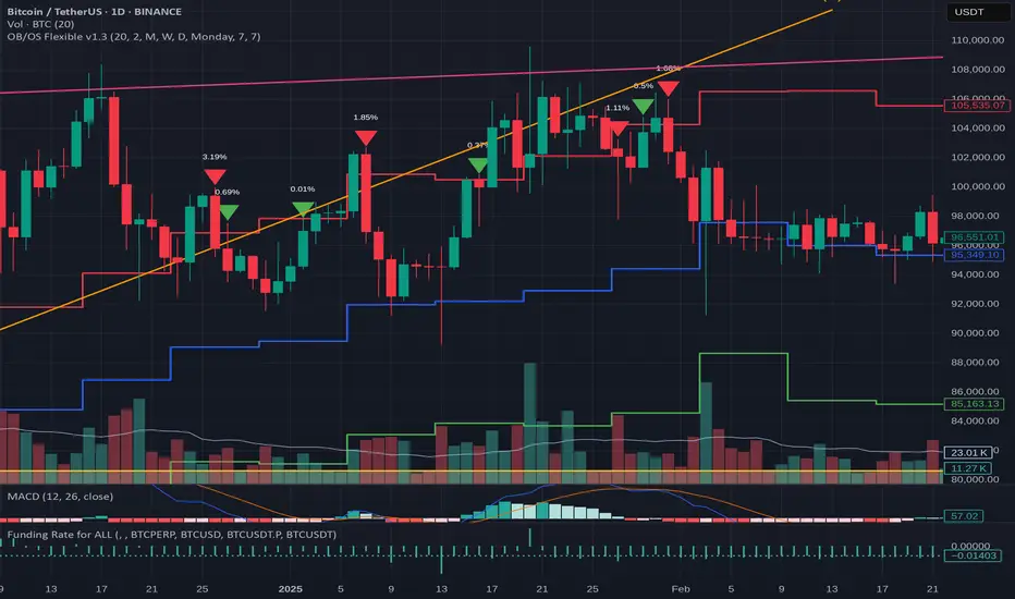
EVaR Indicator and Position SizingThe Problem:
Financial markets consistently show "fat-tailed" distributions where extreme events occur with higher frequency than predicted by normal distributions (Gaussian or even log-normal). These fat tails manifest in sudden price crashes, volatility spikes, and black swan events that traditional risk measures like volatility can underestimate. Standard deviation and conventional VaR calculations assume normally distributed returns, leaving traders vulnerable to severe drawdowns during market stress.
Cryptocurrencies and volatile instruments display particularly pronounced fat-tailed behavior, with extreme moves occurring 5-10 times more frequently than normal distribution models would predict. This reality demands a more sophisticated approach to risk measurement and position sizing.
The Solution: Entropic Value at Risk (EVAR)
EVaR addresses these limitations by incorporating principles from statistical mechanics and information theory through Tsallis entropy. This advanced approach captures the non-linear dependencies and power-law distributions characteristic of real financial markets.
Entropy is more adaptive than standard deviations and volatility measures.
I was inspired to create this indicator after reading the paper " The End of Mean-Variance? Tsallis Entropy Revolutionises Portfolio Optimisation in Cryptocurrencies " by by Sana Gaied Chortane and Kamel Naoui.
Key advantages of EVAR over traditional risk measures:
Superior tail risk capture: More accurately quantifies the probability of extreme market moves
Adaptability to market regimes: Self-calibrates to changing volatility environments
Non-parametric flexibility: Makes less assumptions about the underlying return distribution
Forward-looking risk assessment: Better anticipates potential market changes (just look at the charts :)
Mathematically, EVAR is defined as:
EVAR_α(X) = inf_{z>0} {z * log(1/α * M_X(1/z))}
Where the moment-generating function is calculated using q-exponentials rather than conventional exponentials, allowing precise modeling of fat-tailed behavior.
Technical Implementation
This indicator implements EVAR through a q-exponential approach from Tsallis statistics:
Returns Calculation: Price returns are calculated over the lookback period
Moment Generating Function: Approximated using q-exponentials to account for fat tails
EVAR Computation: Derived from the MGF and confidence parameter
Normalization: Scaled to for intuitive visualization
Position Sizing: Inversely modulated based on normalized EVAR
The q-parameter controls tail sensitivity—higher values (1.5-2.0) increase the weighting of extreme events in the calculation, making the model more conservative during potentially turbulent conditions.
Indicator Components
1. EVAR Risk Visualization
Dynamic EVAR Plot: Color-coded from red to green normalized risk measurement (0-1)
Risk Thresholds: Reference lines at 0.3, 0.5, and 0.7 delineating risk zones
2. Position Sizing Matrix
Risk Assessment: Current risk level and raw EVAR value
Position Recommendations: Percentage allocation, dollar value, and quantity
Stop Parameters: Mathematically derived stop price with percentage distance
Drawdown Projection: Maximum theoretical loss if stop is triggered
Interpretation and Application
The normalized EVAR reading provides a probabilistic risk assessment:
< 0.3: Low risk environment with minimal tail concerns
0.3-0.5: Moderate risk with standard tail behavior
0.5-0.7: Elevated risk with increased probability of significant moves
> 0.7: High risk environment with substantial tail risk present
Position sizing is automatically calculated using an inverse relationship to EVAR, contracting during high-risk periods and expanding during low-risk conditions. This is a counter-cyclical approach that ensures consistent risk exposure across varying market regimes, especially when the market is hyped or overheated.
Parameter Optimization
For optimal risk assessment across market conditions:
Lookback Period: Determines the historical window for risk calculation
Q Parameter: Controls tail sensitivity (higher values increase conservatism)
Confidence Level: Sets the statistical threshold for risk assessment
For cryptocurrencies and highly volatile instruments, a q-parameter between 1.5-2.0 typically provides the most accurate risk assessment because it helps capturing the fat-tailed behavior characteristic of these markets. You can also increase the q-parameter for more conservative approaches.
Practical Applications
Adaptive Risk Management: Quantify and respond to changing tail risk conditions
Volatility-Normalized Positioning: Maintain consistent exposure across market regimes
Black Swan Detection: Early identification of potential extreme market conditions
Portfolio Construction: Apply consistent risk-based sizing across diverse instruments
This indicator is my own approach to entropy-based risk measures as an alterative to volatility and standard deviations and it helps with fat-tailed markets.
Enjoy!

Rolling Log Returns [BackQuant]Rolling Log Returns
The Rolling Log Returns indicator is a versatile tool designed to help traders, quants, and data-driven analysts evaluate the dynamics of price changes using logarithmic return analysis. Widely adopted in quantitative finance, log returns offer several mathematical and statistical advantages over simple returns, making them ideal for backtesting, portfolio optimization, volatility modeling, and risk management.
What Are Log Returns?
In quantitative finance, logarithmic returns are defined as:
ln(Pₜ / Pₜ₋₁)
or for rolling periods:
ln(Pₜ / Pₜ₋ₙ)
where P represents price and n is the rolling lookback window.
Log returns are preferred because:
They are time additive : returns over multiple periods can be summed.
They allow for easier statistical modeling , especially when assuming normally distributed returns.
They behave symmetrically for gains and losses, unlike arithmetic returns.
They normalize percentage changes, making cross-asset or cross-timeframe comparisons more consistent.
Indicator Overview
The Rolling Log Returns indicator computes log returns either on a standard (1-period) basis or using a rolling lookback period , allowing users to adapt it to short-term trading or long-term trend analysis.
It also supports a comparison series , enabling traders to compare the return structure of the main charted asset to another instrument (e.g., SPY, BTC, etc.).
Core Features
✅ Return Modes :
Normal Log Returns : Measures ln(price / price ), ideal for day-to-day return analysis.
Rolling Log Returns : Measures ln(price / price ), highlighting price drift over longer horizons.
✅ Comparison Support :
Compare log returns of the primary instrument to another symbol (like an index or ETF).
Useful for relative performance and market regime analysis .
✅ Moving Averages of Returns :
Smooth noisy return series with customizable MA types: SMA, EMA, WMA, RMA, and Linear Regression.
Applicable to both primary and comparison series.
✅ Conditional Coloring :
Returns > 0 are colored green ; returns < 0 are red .
Comparison series gets its own unique color scheme.
✅ Extreme Return Detection :
Highlight unusually large price moves using upper/lower thresholds.
Visually flags abnormal volatility events such as earnings surprises or macroeconomic shocks.
Quantitative Use Cases
🔍 Return Distribution Analysis :
Gain insight into the statistical properties of asset returns (e.g., skewness, kurtosis, tail behavior).
📉 Risk Management :
Use historical return outliers to define drawdown expectations, stress tests, or VaR simulations.
🔁 Strategy Backtesting :
Apply rolling log returns to momentum or mean-reversion models where compounding and consistent scaling matter.
📊 Market Regime Detection :
Identify periods of consistent overperformance/underperformance relative to a benchmark asset.
📈 Signal Engineering :
Incorporate return deltas, moving average crossover of returns, or threshold-based triggers into machine learning pipelines or rule-based systems.
Recommended Settings
Use Normal mode for high-frequency trading signals.
Use Rolling mode for swing or trend-following strategies.
Compare vs. a broad market index (e.g., SPY or QQQ ) to extract relative strength insights.
Set upper and lower thresholds around ±5% for spotting major volatility days.
Conclusion
The Rolling Log Returns indicator transforms raw price action into a statistically sound return series—equipping traders with a professional-grade lens into market behavior. Whether you're conducting exploratory data analysis, building factor models, or visually scanning for outliers, this indicator integrates seamlessly into a modern quant's toolbox.
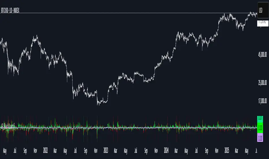
Multi-Timeline 1.0Multi-TimeLines 1.0 - Comprehensive Description
WHAT IT DOES:
This indicator creates dynamic horizontal support/resistance lines based on opening prices captured at user-defined New York times. Unlike static horizontal lines, these levels automatically appear and disappear based on sophisticated session logic, providing traders with time-sensitive reference levels that adapt to market sessions.
HOW IT WORKS - TECHNICAL IMPLEMENTATION:
1.
Timezone Conversion Engine:
The script uses Pine Script's "America/New_York" timezone functions to ensure all time calculations are based on NY time, regardless of the user's chart timezone. This eliminates confusion and provides consistent behavior across global markets.
2.
Dual-Category Time Classification System:
The indicator employs a unique two-category classification system:
Category A (16:00-23:59 NY): Evening times that extend overnight until next day 15:59 NY
Category B (00:00-15:59 NY): Day times that extend until same day 15:59 NY
This classification handles the complex logic of overnight sessions and prevents lines from incorrectly resetting at midnight for evening times.
3. Price Capture Mechanism:
Uses precise time-hit detection with backup systems for edge cases (especially midnight 00:00). When a specified time occurs, the script captures the bar's opening price and stores it in persistent variables using Pine Script's var declarations.
4. Session-Aware Display Logic:
Lines only appear during their designated "display windows" - periods when the captured price level is relevant. The script uses conditional plotting with plot.style_linebr to create clean breaks when lines are inactive.
5. Smart Reset System:
Different reset behaviors based on time classification:
Category A times persist across midnight (for overnight analysis)
Category B times reset on day changes (except 00:00 which captures AT day change)
Automatic cleanup when display windows close
ORIGINALITY & UNIQUE FEATURES:
1. Overnight Session Handling:
Unlike basic horizontal line tools, this script properly handles overnight spans for evening times, making it invaluable for analyzing gaps and overnight price action.
2. Automatic Session Management:
No manual line drawing required - the script automatically manages when lines appear/disappear based on NY market sessions (15:59 close, 18:00 after-hours start).
3. Time-Window Display Logic:
Lines only show during relevant periods, reducing chart clutter and focusing attention on currently active levels.
TRADING CONCEPTS & APPLICATIONS:
1. Session-Based Analysis:
Capture opening prices at key session times:
00:00 NY: Sydney/Asian session start
03:00 NY: London pre-market
08:00 NY: London session open
09:30 NY: NYSE opening bell
18:00 NY: After-hours start
2. Gap Analysis:
Evening times (20:00-23:59) that extend overnight are particularly useful for:
Identifying potential gap-fill levels
Tracking overnight high/low breaks
Setting reference points for next-day trading
3. Support/Resistance Framework:
Opening prices at significant times often act as:
Intraday support/resistance levels
Reference points for breakout/breakdown analysis
Pivot levels for mean reversion strategies
HOW TO USE:
1. Time Input:
Enter times in "HH:MM" format using 24-hour NY time:
"09:30" for NYSE open
"15:30" for late-day reference
"20:00" for evening level (extends overnight)
2. Line Behavior:
Blue/Green/Cyan/Red lines: Your custom times
Yellow line: After-hours day open (18:00 NY start)
Lines appear with breaks during inactive periods
3. Strategic Setup:
Use 2-3 key session times for your trading style
Combine morning times (immediate reference) with evening times (overnight analysis)
Toggle after-hours line based on your market focus
CALCULATION METHOD:
The script uses direct opening price capture (no smoothing or averaging) at precise time hits, ensuring the most accurate representation of actual market levels at specified times. This raw price approach maintains the integrity of actual market opening prices rather than manipulated or calculated values.
This method is particularly effective because opening prices at significant times often represent institutional order flow and can act as magnetic levels throughout subsequent sessions.
