Customizable BTC Seasonality StrategyThis strategy leverages intraday seasonality effects in Bitcoin, specifically targeting hours of statistically significant returns during periods when traditional financial markets are closed. Padysak and Vojtko (2022) demonstrate that Bitcoin exhibits higher-than-average returns from 21:00 UTC to 23:00 UTC, a period in which all major global exchanges, such as the New York Stock Exchange (NYSE), Tokyo Stock Exchange, and London Stock Exchange, are closed. The absence of competing trading activity from traditional markets during these hours appears to contribute to these statistically significant returns.
The strategy proceeds as follows:
Entry Time: A long position in Bitcoin is opened at a user-specified time, which defaults to 21:00 UTC, aligning with the beginning of the identified high-return window.
Holding Period: The position is held for two hours, capturing the positive returns typically observed during this period.
Exit Time: The position is closed at a user-defined time, defaulting to 23:00 UTC, allowing the strategy to exit as the favorable period concludes.
This simple seasonality strategy aims to achieve a 33% annualized return with a notably reduced volatility of 20.93% and maximum drawdown of -22.45%. The results suggest that investing only during these high-return hours is more stable and less risky than a passive holding strategy (Padysak & Vojtko, 2022).
References
Padysak, M., & Vojtko, R. (2022). Seasonality, Trend-following, and Mean reversion in Bitcoin.
Wyszukaj w skryptach "[中国保险行业协会]:2022年度商业健康保险经营数据"

Economic Calendar (Import from Spreadsheet)This script draws vertical lines to mark Economic Calendar Events.
Datetime of events is defined by user in Settings via a standardized line of text.
Motivation for coding this script:
All traders should be aware of economic calendar events. At times, when you really need to pay attention to an upcoming major event, you might even decide to use the vertical-line drawing tool to mark it. However, this takes manual effort.
This script provides a solution to performing mundane tasks such as drawing vertical lines and dragging them ever so slightly, just to have them approximately aligned with exact time.
Parameters:
(1) Source data - String representation of collection of datetime referencing to Economic Calendar Events
(2) Line color, & (3) Width of line - For displaying vertical lines drawn by script.
Standardized format for Source Data :
Example:
If 'GMT;2022,6,1,14,0,0;2022,6,2,12,15,0;' is provided to PineScript, then two vertical lines will be drawn on June 6, 2022 according to the exact time in 'YYYY,MM,DD,hh,mm,ss' format at the specified timezone (GMT in this case).
Template for Source Data :
Included here, link below, is a shared Google Sheet that systematically processes Economic Calendar data provided in the 'Raw Data' tab.
drive.google.com
Users are advised to use their preferred methods* to format the string (for source data param.), and apply their own criteria to sort down the Events. (ie. only include Events of High Impact, etc.)
* Preferred methods (as mentioned above) does not mean being limited to using the template as provided in this post.

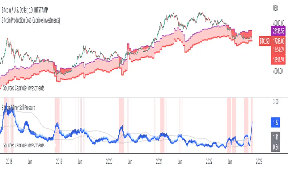
Bitcoin Miner Sell PressureBitcoin miners are in pain and now (November 2022) selling more than they have in almost 5 years!
Introducing: Bitcoin Miner Sell Pressure.
A free, open-source indicator which tracks on-chain data to highlight when Bitcoin miners are selling more of their reserves than usual.
The indicator tracks the ratio of on-chain miner Bitcoin outflows to miner Bitcoin reserves.
- Higher = more selling than usual
- Lower = less selling than usual
- Red = extraordinary sell pressure
Today , it's red.
What can we see now ?
Miners are not great at treasury management. They tend to sell most when they are losing money (like today). But there have been times when they sold well into high profit, such as into the 2017 $20K top and in early 2021 when Bitcoin breached $40K.
Bitcoin Miner Sell Pressure identifies industry stress, excess and miner capitulation.
Unsurprisingly, there is a high correlation with Bitcoin Production Cost; giving strong confluence to both.
In some instances, BMSP spots capitulation before Hash Ribbons. Such as today!
Yearly Monthly Vertical Lines [MsF]This indicator that draws vertical lines for each year and month starting from the specified date and time.
For example, starting from August 26th, 2022,
The annual vertical lines are Aug 26th, 2022, Aug 26th, 2021, Aug 26th, 2020, Aug 26th, 2019, Aug 26th, 2018, Aug 26th, 2017...
It is useful to check the action of the chart at the event of each year and month.
Caution:
Since there is a limit to the Bar-Count that can be specified in the script language, depending on the chart period setting It may not be displayed.
-------------------------
指定した日時を起点として、年、月ごとに垂直線(縦線)を描画するインジケータです。
例えば、2022/9/1を起点とした場合、
年次のラインは、2021/9/1、2020/9/1、2019/9/1、2018/9/1、2017/9/1、2016/9/1...
に描画します。
年、月ごとのイベント時のチャートの動きを確認するのに便利です。
※過去イベント時の価格変動確認の際、手作業で垂直線を引くのが面倒なため、作成しました。
<注意>
スクリプト言語で指定できるBarCntに制限がある為、チャートの期間設定によっては
表示されない場合があります。※今後改善の余地あり

[HA] Heikin-Ashi Shadow Candles// For overlaying Heikin Ashi candles over basic charts, or for use in it's own panel as an oscillator.
// Enjoy the visual cues of HA candles, without giving up price action awareness.
// Good for learning and comparison.
// Aug 11 2022
Release Notes: * Bugfix: Candle color was based on classic direction not HA direction (did not update cover photo).
// Aug 12 2022
Release Notes: * Implemented true oscillator mode.
Provided as separate plot (styles tab) or mode switch option (Inputs tab). TV gets spazzy with "styles tab" "default hidden" plots, and will reset them if any variables are modified that affect them (i.e. wick color override). Mode switch should be sufficient for both users.
// Aug 21 2022
Republished because of typo in indicator name prevented search.

Inverse MACD + DMI Scalping with Volatility Stop (By Coinrule)This script is focused on shorting during downtrends and utilises two strength based indicators to provide confluence that the start of a short-term downtrend has occurred - catching the opportunity as soon as possible.
This script can work well on coins you are planning to hodl for long-term and works especially well whilst using an automated bot that can execute your trades for you. It allows you to hedge your investment by allocating a % of your coins to trade with, whilst not risking your entire holding. This mitigates unrealised losses from hodling as it provides additional cash from the profits made. You can then choose to hodl this cash, or use it to reinvest when the market reaches attractive buying levels.
Alternatively, you can use this when trading contracts on futures markets where there is no need to already own the underlying asset prior to shorting it.
ENTRY
The trading system uses the Momentum Average Convergence Divergence (MACD) indicator and the Directional Movement Index (DMI) indicator to confirm when the best time is for selling. Combining these two indicators prevents trading during uptrends and reduces the likelihood of getting stuck in a market with low volatility.
The MACD is a trend following momentum indicator and provides identification of short-term trend direction. In this variation it utilises the 12-period as the fast and 26-period as the slow length EMAs, with signal smoothing set at 9.
The DMI indicates what way price is trending and compares prior lows and highs with two lines drawn between each - the positive directional movement line (+DI) and the negative directional movement line (-DI). The trend can be interpreted by comparing the two lines and what line is greater. When the negative DMI is greater than the positive DMI, there are more chances that the asset is trading in a sustained downtrend, and vice versa.
The system will enter trades when two conditions are met:
1) The MACD histogram turns bearish.
2) When the negative DMI is greater than the positive DMI.
EXIT
The strategy comes with a fixed take profit combined with a volatility stop, which acts as a trailing stop to adapt to the trend's strength. Depending on your long-term confidence in the asset, you can edit the fixed take profit to be more conservative or aggressive.
The position is closed when:
Take-Profit Exit: +8% price decrease from entry price.
OR
Stop-Loss Exit: Price crosses above the volatility stop.
In general, this approach suits medium to long term strategies. The backtesting for this strategy begins on 1 April 2022 to 18 July 2022 in order to demonstrate its results in a bear market. Back testing it further from the beginning of 2022 onwards further also produces good returns.
Pairs that produce very strong results include SOLUSDT on the 45m timeframe, MATICUSDT on the 2h timeframe, and AVAUSDT on the 1h timeframe. Generally, the back testing suggests that it works best on the 45m/1h timeframe across most pairs.
A trading fee of 0.1% is also taken into account and is aligned to the base fee applied on Binance.

Gold and Bitcoin: The Evolution of Value!The Eternal Luster of Gold
In the dawn of time, when the earth was young and rivers whispered secrets to the stones, a wanderer named Elara found a gleam in the silt of a sun-kissed stream. It was pure gold, radiant like a captured star fallen from the heavens. She held it in her palm, feeling its warmth pulse like a heartbeat, and in that moment, humanity’s soul awakened to the allure of eternity.
As seasons turned to centuries, gold wove itself into the story of empires. In ancient Egypt, pharaohs crowned themselves with its glow, believing it to be the flesh of gods. It built pyramids that reached for the sky and tombs that guarded kings forever. Across the sands in Mesopotamia, merchants traded it for spices and silks, its weight a promise of power and trust.
Translation moment: Gold became the first universal symbol of value. People trusted it more than words or promises because it did not rust, fade, or vanish.
The Greeks saw in gold not only wealth but wisdom, the symbol of the sun’s eternal fire. Alexander the Great carried it across the continent, forging an empire of golden threads. Rome rose on its back, minting coins whose clink echoed through history.
Through the ages, gold endured the rush of California’s dreamers, the halls of Versailles, and the quiet vaults of modern fortunes. It has been both a curse and a blessing, the fuel of wars and the gift of love, whispering of beauty’s fragility and the human desire for something that lasts beyond the grave. In its shine, we see ourselves fragile yet forever chasing light.
The Digital Dawn of Bitcoin
Centuries later, under the glow of computer screens, a visionary named Satoshi dreamed of a new gold born not from the earth but from the ether of ideas. Bitcoin appeared in 2009 amid a world weary of banks and broken trust.
Like gold’s ancient gleam, Bitcoin was mined not with picks but with puzzles solved by machines. It promised freedom, a currency without kings, flowing from person to person, unbound by borders or empires.
Translation moment: Bitcoin works like digital gold. Instead of digging the ground, miners use computers to solve problems and unlock new coins. No one controls it, and that is what makes it powerful.
Through doubt and frenzy, it rose as a beacon for those seeking sovereignty in a digital world. Its volatility became its soul, a reminder that true value is built on belief. Bitcoin speaks to ingenuity and rebellion, a star of code guiding us toward a future where wealth is weightless yet profoundly honest.
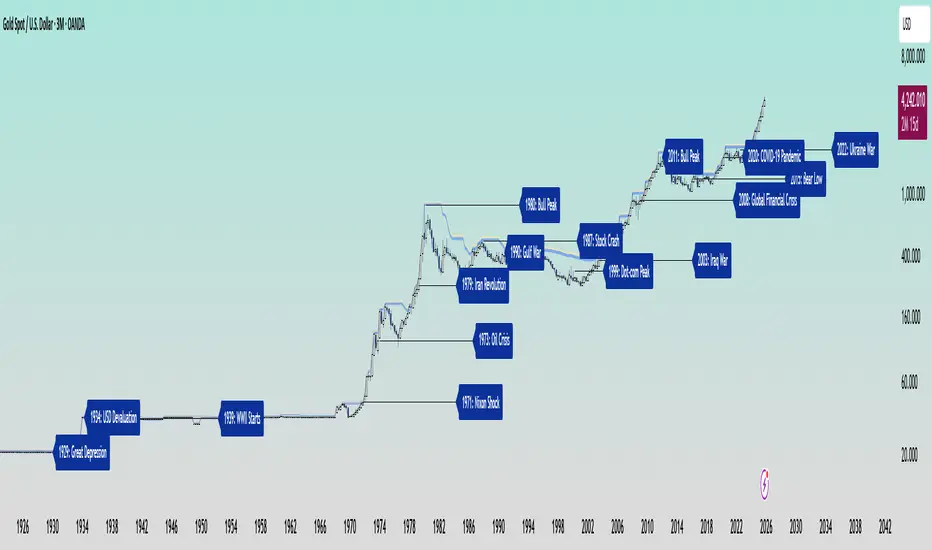
Gold’s Cycles: Echoes of War and Crisis
In the early 20th century, gold was held under fixed prices until the Great Depression of 1929 shattered these illusions. The 1934 dollar devaluation lifted it from 20.67 to 35, restoring faith amid despair. When World War II erupted in 1939, gold’s role as a refuge was muted by controls, yet it quietly held its place as the world’s silent guardian.
The 1970s awakened its wild spirit. The Nixon Shock of 1971 freed gold from 35, sparking a bull run during the 1973 Oil Crisis. The 1979 Iranian Revolution led to a 1980 peak of 850, a leap of more than 2,000 percent, as investors sought safety from the chaos.
Translation moment: When fear rises, people rush to gold. Every major war or economic crisis has sent gold upward because it feels safe when paper money loses trust.
The 1987 stock crash caused brief dips, but the 1990 Gulf War reignited its glow. Around 2000, after the Dot-com Bust, gold found new life, climbing from $ 270 to over $1,900 during the 2008 Financial Crisis. It dipped to 1050 in 2015, then surged again past 2000 during the 2020 pandemic.
The 2022 Ukraine War added another chapter with prices climbing above 2700 by 2025. Across a century of crises, gold has risen whenever fear tested humanity’s resolve, teaching patience and fortitude through its quiet endurance.
Bitcoin’s Cycles: Echoes of Innovation and Crisis
Born from the ashes of the 2008 Financial Crisis, Bitcoin began its story at mere cents. It traded below $1 until 2011, when it reached $30 before crashing by 90 percent following the MTGOX collapse.
In 2013, it soared to 1242 only to fall again to 200 in 2015 as regulations tightened. The 2017 bull run lifted it to nearly 20000 before another long winter brought it to 3200 in 2018. Each fall taught resilience, each rise renewed belief.
During the 2020 pandemic, it fell below 5000 before rallying to 69000 in 2021. The Ukraine War and the FTX collapse of 2022 brought it down to 16000, but also proved its role in humanitarian aid. By 2024, the halving and ETF approvals helped it break 100000, marking Bitcoin’s rise as digital gold.
Translation moment: Bitcoin’s rhythm follows four-year halving cycles when mining rewards are cut in half. This keeps supply limited, which often triggers new bull runs as demand returns.
Every four years, it's halving cycles 2012, 2016, 2020, 2024, fueling new waves of adoption and correction. Bitcoin grows strongest in times of uncertainty, echoing humanity’s drive to evolve beyond limits.
The Harmony of Gold and Bitcoin Modern Parallels
In today’s markets, gold’s ancient glow meets Bitcoin’s electric pulse. As of October 17, 2025, their correlation stands near 0.85, close to its historic high of 0.9. Both rise as guardians against inflation and the erosion of trust in the dollar.
Gold trades near 4310 per ounce a record high while Bitcoin hovers around 104700 showing brief fractures in their unity. Gold offers the comfort of touch while Bitcoin provides the thrill of code. Together, they reflect fear and hope, the twin emotions that drive every market.
Translation moment: A correlation of 0.85 means they often move in the same direction. When fear or inflation rises, both gold and Bitcoin tend to rise in tandem.
Analysts warn of bubbles in stocks, gold, and crypto, yet optimism remains for Bitcoin’s growth through 2026, while gold holds its defensive strength.
Gold carries risks of storage cost and theft, but steadiness in chaos. Bitcoin carries volatility and regulatory challenges, but it also offers unmatched innovation and reach. One is the anchor, the other the dream, and both reward those who hold conviction through uncertainty.
Epilogue: The Timeless Balance
Gold and Bitcoin form a bridge between the ancient and the future. Gold, the earth’s eternal treasure, stands as a symbol of stability and truth. Bitcoin, the digital heir, shines with the spark of innovation and freedom.
Experts view gold as the ultimate inflation hedge, forged in fire and tested over centuries. They see Bitcoin as its digital counterpart, scarce by code and limitless in reach.
Gold’s weight grounds us in reality while Bitcoin’s light expands our imagination. In 2025, as gold surpasses $4,346 and Bitcoin hovers near $105,000, the wise investor sees not rivals but reflections.
Translation moment: Gold reminds us to protect what we have. Bitcoin reminds us to dream of what could be. Together, they balance caution and courage, the two forces every generation must master.
One whispers of legacy, the other of evolution, yet together they tell humanity’s oldest story, our unending quest to preserve value against time and to chase the light that never fades.
🙏 I ask (Allah) for guidance and success. 🤲
Ethereum Logarithmic Regression BandsOverview
This indicator displays logarithmic regression bands for Ethereum. Logarithmic regression is a statistical method used to model data where growth slows down over time. I initially created these bands in 2021 using a spreadsheet, and later coded them in TradingView in 2022. Over time, the bands proved effective at capturing bull market peaks and bear market lows. In 2025, I decided to share this indicator because I believe these logarithmic regression bands offer the best fit for the Ethereum chart.
How It Works
The logarithmic regression lines are fitted to the Ethereum (ETHUSD) chart using two key factors: the 'a' factor (slope) and the 'b' factor (intercept). The formula for logarithmic regression is 10^((a * ln) - b).
How to Use the Logarithmic Regression Bands
1. Lower Band:
The lower (blue) band forms a potential support area for Ethereum’s price. Historically, Ethereum has found its lows within this band during past market cycles. When the price is within the lower band, it suggests that Ethereum is undervalued.
2. Upper Band:
The upper (red) band forms a potential resistance area for Ethereum’s price. The logarithmic band is fitted to the past two market cycle peaks; therefore, there is not enough historical data to be sure it will reach the upper band again. However, the chance is certainly there! If the price is within the upper band, it indicates that Ethereum is overvalued and that a potential price correction may be imminent.

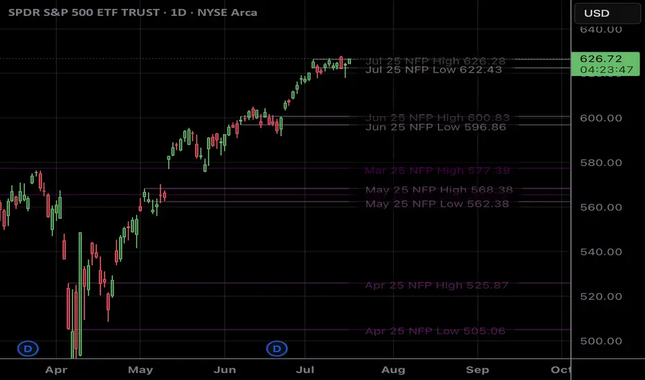
NFP RangesPlots the NFP daily ranges for NFP days. Includes extended hours ranges when the time frame is sub 1D, otherwise, only the daily range is taken.
NFP Dates are pre-populated through 2029 and historically through 2022. Will update script to include farther-out dates before they become necessary.
JPMorgan G7 Volatility IndexThe JPMorgan G7 Volatility Index: Scientific Analysis and Professional Applications
Introduction
The JPMorgan G7 Volatility Index (G7VOL) represents a sophisticated metric for monitoring currency market volatility across major developed economies. This indicator functions as an approximation of JPMorgan's proprietary volatility indices, providing traders and investors with a normalized measurement of cross-currency volatility conditions (Clark, 2019).
Theoretical Foundation
Currency volatility is fundamentally defined as "the statistical measure of the dispersion of returns for a given security or market index" (Hull, 2018, p.127). In the context of G7 currencies, this volatility measurement becomes particularly significant due to the economic importance of these nations, which collectively represent more than 50% of global nominal GDP (IMF, 2022).
According to Menkhoff et al. (2012, p.685), "currency volatility serves as a global risk factor that affects expected returns across different asset classes." This finding underscores the importance of monitoring G7 currency volatility as a proxy for global financial conditions.
Methodology
The G7VOL indicator employs a multi-step calculation process:
Individual volatility calculation for seven major currency pairs using standard deviation normalized by price (Lo, 2002)
- Weighted-average combination of these volatilities to form a composite index
- Normalization against historical bands to create a standardized scale
- Visual representation through dynamic coloring that reflects current market conditions
The mathematical foundation follows the volatility calculation methodology proposed by Bollerslev et al. (2018):
Volatility = σ(returns) / price × 100
Where σ represents standard deviation calculated over a specified timeframe, typically 20 periods as recommended by the Bank for International Settlements (BIS, 2020).
Professional Applications
Professional traders and institutional investors employ the G7VOL indicator in several key ways:
1. Risk Management Signaling
According to research by Adrian and Brunnermeier (2016), elevated currency volatility often precedes broader market stress. When the G7VOL breaches its high volatility threshold (typically 1.5 times the 100-period average), portfolio managers frequently reduce risk exposure across asset classes. As noted by Borio (2019, p.17), "currency volatility spikes have historically preceded equity market corrections by 2-7 trading days."
2. Counter-Cyclical Investment Strategy
Low G7 volatility periods (readings below the lower band) tend to coincide with what Shin (2017) describes as "risk-on" environments. Professional investors often use these signals to increase allocations to higher-beta assets and emerging markets. Campbell et al. (2021) found that G7 volatility in the lowest quintile historically preceded emerging market outperformance by an average of 3.7% over subsequent quarters.
3. Regime Identification
The normalized volatility framework enables identification of distinct market regimes:
- Readings above 1.0: Crisis/high volatility regime
- Readings between -0.5 and 0.5: Normal volatility regime
- Readings below -1.0: Unusually calm markets
According to Rey (2015), these regimes have significant implications for global monetary policy transmission mechanisms and cross-border capital flows.
Interpretation and Trading Applications
G7 currency volatility serves as a barometer for global financial conditions due to these currencies' centrality in international trade and reserve status. As noted by Gagnon and Ihrig (2021, p.423), "G7 currency volatility captures both trade-related uncertainty and broader financial market risk appetites."
Professional traders apply this indicator in multiple contexts:
- Leading indicator: Research from the Federal Reserve Board (Powell, 2020) suggests G7 volatility often leads VIX movements by 1-3 days, providing advance warning of broader market volatility.
- Correlation shifts: During periods of elevated G7 volatility, cross-asset correlations typically increase what Brunnermeier and Pedersen (2009) term "correlation breakdown during stress periods." This phenomenon informs portfolio diversification strategies.
- Carry trade timing: Currency carry strategies perform best during low volatility regimes as documented by Lustig et al. (2011). The G7VOL indicator provides objective thresholds for initiating or exiting such positions.
References
Adrian, T. and Brunnermeier, M.K. (2016) 'CoVaR', American Economic Review, 106(7), pp.1705-1741.
Bank for International Settlements (2020) Monitoring Volatility in Foreign Exchange Markets. BIS Quarterly Review, December 2020.
Bollerslev, T., Patton, A.J. and Quaedvlieg, R. (2018) 'Modeling and forecasting (un)reliable realized volatilities', Journal of Econometrics, 204(1), pp.112-130.
Borio, C. (2019) 'Monetary policy in the grip of a pincer movement', BIS Working Papers, No. 706.
Brunnermeier, M.K. and Pedersen, L.H. (2009) 'Market liquidity and funding liquidity', Review of Financial Studies, 22(6), pp.2201-2238.
Campbell, J.Y., Sunderam, A. and Viceira, L.M. (2021) 'Inflation Bets or Deflation Hedges? The Changing Risks of Nominal Bonds', Critical Finance Review, 10(2), pp.303-336.
Clark, J. (2019) 'Currency Volatility and Macro Fundamentals', JPMorgan Global FX Research Quarterly, Fall 2019.
Gagnon, J.E. and Ihrig, J. (2021) 'What drives foreign exchange markets?', International Finance, 24(3), pp.414-428.
Hull, J.C. (2018) Options, Futures, and Other Derivatives. 10th edn. London: Pearson.
International Monetary Fund (2022) World Economic Outlook Database. Washington, DC: IMF.
Lo, A.W. (2002) 'The statistics of Sharpe ratios', Financial Analysts Journal, 58(4), pp.36-52.
Lustig, H., Roussanov, N. and Verdelhan, A. (2011) 'Common risk factors in currency markets', Review of Financial Studies, 24(11), pp.3731-3777.
Menkhoff, L., Sarno, L., Schmeling, M. and Schrimpf, A. (2012) 'Carry trades and global foreign exchange volatility', Journal of Finance, 67(2), pp.681-718.
Powell, J. (2020) Monetary Policy and Price Stability. Speech at Jackson Hole Economic Symposium, August 27, 2020.
Rey, H. (2015) 'Dilemma not trilemma: The global financial cycle and monetary policy independence', NBER Working Paper No. 21162.
Shin, H.S. (2017) 'The bank/capital markets nexus goes global', Bank for International Settlements Speech, January 15, 2017.

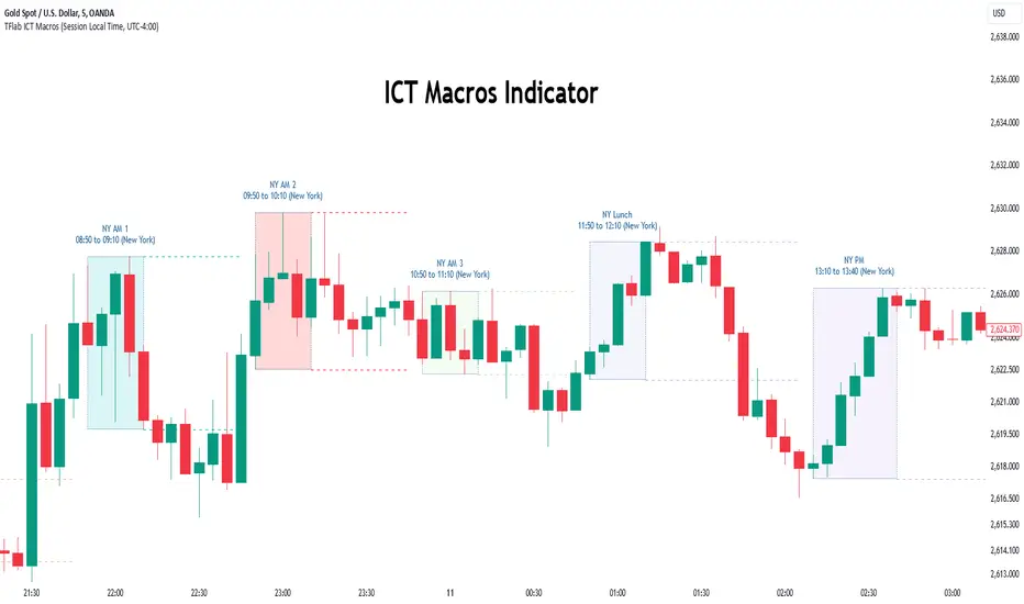
Macros ICT KillZones [TradingFinder] Times & Price Trading Setup🔵 Introduction
ICT Macros, developed by Michael Huddleston, also known as ICT (Inner Circle Trader), is a powerful trading tool designed to help traders identify the best trading opportunities during key time intervals like the London and New York trading sessions.
For traders aiming to capitalize on market volatility, liquidity shifts, and Fair Value Gaps (FVG), understanding and using these critical time zones can significantly improve trading outcomes.
In today’s highly competitive financial markets, identifying the moments when the market is seeking buy-side or sell-side liquidity, or filling price imbalances, is essential for maximizing profitability.
The ICT Macros indicator is built on the renowned ICT time and price theory, which enables traders to track and leverage key market dynamics such as breaks of highs and lows, imbalances, and liquidity hunts.
This indicator automatically detects crucial market times and optimizes strategies for traders by highlighting the specific moments when price movements are most likely to occur. A standout feature of ICT Macros is its automatic adjustment for Daylight Saving Time (DST), ensuring that traders remain synced with the correct session times.
This means you can rely on accurate market timing without the need for manual updates, allowing you to focus on capturing profitable trades during critical timeframes.
🔵 How to Use
The ICT Macros indicator helps you capitalize on trading opportunities during key market moments, particularly when the market is breaking highs or lows, filling Fair Value Gaps (FVG), or addressing imbalances. This indicator is particularly beneficial for traders who seek to identify liquidity, market volatility, and price imbalances.
🟣 Sessions
London Sessions
London Macro 1 :
UTC Time : 06:33 to 07:00
New York Time : 02:33 to 03:00
London Macro 2 :
UTC Time : 08:03 to 08:30
New York Time : 04:03 to 04:30
New York Sessions
New York Macro AM 1 :
UTC Time : 12:50 to 13:10
New York Time : 08:50 to 09:10
New York Macro AM 2 :
UTC Time : 13:50 to 14:10
New York Time : 09:50 to 10:10
New York Macro AM 3 :
UTC Time : 14:50 to 15:10
New York Time : 10:50 to 11:10
New York Lunch Macro :
UTC Time : 15:50 to 16:10
New York Time : 11:50 to 12:10
New York PM Macro :
UTC Time : 17:10 to 17:40
New York Time : 13:10 to 13:40
New York Last Hour Macro :
UTC Time : 19:15 to 19:45
New York Time : 15:15 to 15:45
These time intervals adjust automatically based on Daylight Saving Time (DST), helping traders to enter or exit trades during key market moments when price volatility is high.
Below are the main applications of this tool and how to incorporate it into your trading strategies :
🟣 Combining ICT Macros with Trading Strategies
The ICT Macros indicator can easily be used in conjunction with various trading strategies. Two well-known strategies that can be combined with this indicator include:
ICT 2022 Trading Model : This model is designed based on identifying market liquidity, structural price changes, and Fair Value Gaps (FVG). By using ICT Macros, you can identify the key time intervals when the market is seeking liquidity, filling imbalances, or breaking through important highs and lows, allowing you to enter or exit trades at the right moment.
Silver Bullet Strategy : This strategy, which is built around liquidity hunting and rapid price movements, can work more accurately with the help of ICT Macros. The indicator pinpoints precise liquidity times, helping traders take advantage of market shifts caused by filling Fair Value Gaps or correcting imbalances.
🟣 Capitalizing on Price Volatility During Key Times
Large market algorithms often seek liquidity or fill Fair Value Gaps (FVG) during the intervals marked by ICT Macros. These periods are when price volatility increases, and traders can use these moments to enter or exit trades.
For example, if sell-side liquidity is drained and the market fills an imbalance, the price might move toward buy-side liquidity. By identifying these moments, which may also involve breaking a previous high or low, you can leverage rapid market fluctuations to your advantage.
🟣 Identifying Liquidity and Price Imbalances
One of the important uses of ICT Macros is identifying points where the market is seeking liquidity and correcting imbalances. You can determine high or low liquidity levels in the market before each ICT Macro, as well as Fair Value Gaps (FVG) and price imbalances that need to be filled, using them to adjust your trading strategy. This capability allows you to manage trades based on liquidity shifts or imbalance corrections without needing a bias toward a specific direction.
🔵 Settings
The ICT Macros indicator offers various customization options, allowing users to tailor it to their specific needs. Below are the main settings:
Time Zone Mode : You can select one of the following options to define how time is displayed:
UTC : For traders who need to work with Universal Time.
Session Local Time : The local time corresponding to the London or New York markets.
Your Time Zone : You can specify your own time zone (e.g., "UTC-4:00").
Your Time Zone : If you choose "Your Time Zone," you can set your specific time zone. By default, this is set to UTC-4:00.
Show Range Time : This option allows you to display the time range of each session on the chart. If enabled, the exact start and end times of each interval are shown.
Show or Hide Time Ranges : Toggle on/off for visual clarity depending on user preference.
Custom Colors : Set distinct colors for each session, allowing users to personalize their chart based on their trading style.These settings allow you to adjust the key time intervals of each trading session to your preference and customize the time format according to your own needs.
🔵 Conclusion
The ICT Macros indicator is a powerful tool for traders, helping them to identify key time intervals where the market seeks liquidity or fills Fair Value Gaps (FVG), corrects imbalances, and breaks highs or lows. This tool is especially valuable for traders using liquidity-based strategies such as ICT 2022 or Silver Bullet.
One of the key features of this indicator is its support for Daylight Saving Time (DST), ensuring you are always in sync with the correct trading session timings without manual adjustments. This is particularly beneficial for traders operating across different time zones.
With ICT Macros, you can capitalize on crucial market opportunities during sensitive times, take advantage of imbalances, and enhance your trading strategies based on market volatility, liquidity shifts, and Fair Value Gaps.
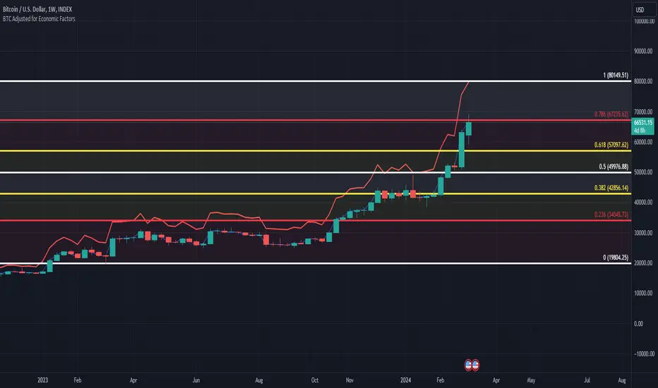
BTC/USD Inflation priced in! ~Period 2009 - 2023 (by TAS)The script creates a custom indicator titled "BTC Adjusted for Economic Factors.
Adjusted BTC Price is plotted in red, making it more prominent. The adjusted price is Bitcoin's historical closing prices adjusted for cumulative inflation over time, based on the Core Consumer Price Index (CPI) annual inflation rates from 2009 onwards.
The script calculates the adjusted price of Bitcoin by taking into account the effect of inflation on its value. It uses annual CPI rates for each year from 2009 to 2022 to calculate a cumulative inflation factor. The script assumes a placeholder inflation rate of 2.5% for 2023, indicating that this value should be updated when the actual rate is available. The script suggests adding CPI rates for additional years as they become available to maintain the accuracy of the adjustment.
Here's a breakdown of how the script works:
Core CPI Annual Inflation Rates: It starts by defining the annual inflation rates for each year from 2009 to 2022, expressed as a percentage divided by 100 to convert to a decimal.
Cumulative Inflation Calculation: The script calculates cumulative inflation starting from the year 2009 up to the current year. For each year that has passed since 2009, it multiplies the cumulative inflation factor by (1 + cpiRate), where cpiRate is the inflation rate for that year. This effectively compounds the inflation rate over time.
Adjusting Bitcoin's Price: The script then adjusts Bitcoin's closing price (close) for the calculated cumulative inflation to get the adjusted price (adjustedPrice).
Plotting the Prices: Finally, it plots both the original and the adjusted Bitcoin prices on the chart, allowing users to visually compare how inflation has theoretically impacted Bitcoin's value over time.
--------------------------------------------------------------------------------------------------
Important to notice, Fib. Retracements from the 2017 cycle top to the recent top (¬80K) doesn't look invalidated.
--------------------------------------------------------------------------------------------------
Inputs and feedback are welcome!
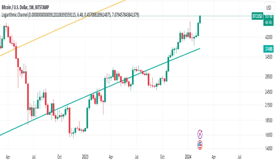
Bitcoin's Logarithmic ChannelLogarithmic growth is a reasonable way to describe the long term growth of bitcoin's market value: for a network that is experiencing growing adoption and is powered by an asset with a finite and disinflationary supply, it’s natural to expect a more explosive growth of its market capitalization early on, followed by diminishing returns as the network and the asset mature.
I used publicly available data to model the market capitalization of bitcoin, deriving thereform a set of three curves forming a logarithmic growth channel for the market capitalization of bitcoin. Using the time series for the circulating supply, we derive a logarithmic growth channel for the bitcoin price.
Model uses publicly available data from July 17, 2010 to December 31, 2022. Everything since the beginning of 2023 is a prediction.
Past performance is not a guarantee of future results.
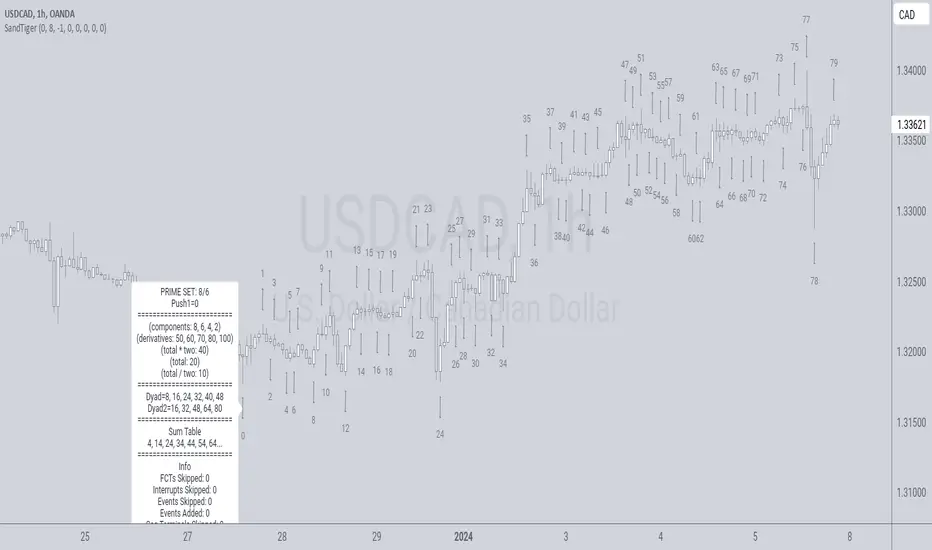
SandTigerSandTiger is an auto-counting tool that counts naturally occurring events in a price series. This version has been reduced to 377 lines of code and should run faster than previous versions. Although not shown here, I highly recommend running my 'ELB' script with SandTiger. ELB is an 'event locator' and will mark all points that SandTiger numbers - giving you visual cues as to where these points are located. ELB also displays support/resistance levels.
SandTiger is designed to be used with MAGENTA - a counting system for Forex and other markets.
MAGENTA is a free and open framework for understanding and explaining price movement in financial markets. Any materials associated with MAGENTA are strictly for educational purposes only.
SandTiger tracks Component Values, Dyads, and Sum Table Values (STV's) over straight and curved trends, allowing a trader to discern where directional shifts are likely to occur.
SandTiger requires just 3 things to function accurately:
1) A correct starting point (this will typically be an obvious trend turn high or low in a series of price moves).
2) A 'push 1' count ('push 1' runs from the starting point to the event prior to the first terminal of the first FCT or Fractured Counter-Trend).
3) A 'high prime' value (the high prime count runs from the starting point through to the second terminal of the first FCT with no skips).
FRAMEWORK OVERVIEW: 'Component' values are filtered from the prime set (including the half prime and further reductions). Once we have the comp table we add the values to get a 'total'. With the 'total' we divide and multiply by two to get two additional values. 'Derivatives' are based on various calculations using these three values.
We're looking for 'total/2' to count into either itself, 'total', 'total*2', or a derivative. Comp counts are in Tx form and counted from trend start. If the trend doesn't turn on a comp value it will likely turn on a Dyad or STV value. If that also doesn't happen it's likely you have a 'curved' trend/sequence that will turn on one of the above after moving away from its high/low. This can also be traded using SandTiger's 'Seg Terminals' skip option.
Sum tables and Dyad values are drawn from the 'primes' and Dyads use the 'push1' value as well. In a structural trend, primes are gotten by counting pushpulls 1 & 2 in 'Ti' form. Comps, Sum table values, and Dyads are equivalent, sequences can turn on either value type belonging to the 1st or 2nd prime set. Both STV's and Dyads are counted in 'Tx' form (except where count-through signals occur).
Types and antitypes correlate and are associated with a 12-count 'cycle.' (Ti = 'Terminals Included'; Tx = 'Terminals eXcluded'; both refer to FCT terminals)
THE STRATEGY:
For Structures: Trade Comps, Dyads, and STV's from sets 1 (all) and 2 (Dyads and STV's only) in the 'main' segment then on the 'carry-over' by skipping segment terminals. If a PC or cycle caps the sequence, trade that as well.
For NSM's: Trade movements that flash a signal prior to the end of the initial cycle. The mark will be the push1 value. Twelve will be the 'high prime.' Skip interrupts and trade carry-over values.
The first version of SandTiger was conceived/planned/authored by Erek A.D. and coded by Erek A.D. and @SimpleCryptoLife beginning in August 2022 and finishing in Dec. 2022
The current version was written and developed July 3, 2023 and has been refined and upgraded by Erek A.D. through Jan. 2024...
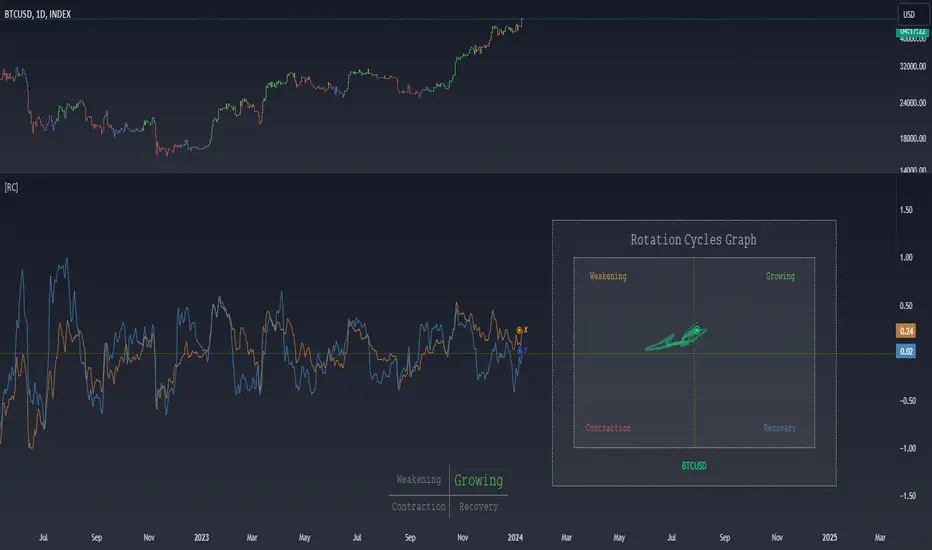
Rotation Cycles GraphRotation Cycles Graph Indicator
Overview:
The Rotation Cycles Graph Indicator is designed to visualize rotation cycles in financial markets. It aims to provide insights into shifts between various market phases, including growth, weakening, recovery, and contraction, allowing traders to potentially identify changing market dynamics.
Key Components:
Z-Score Calculation:
The indicator employs Z-score calculation to normalize data and identify deviations from the mean. This is instrumental in understanding the current state of the market relative to its historical behavior.
Ehlers Loop Visualization:
The Ehlers Loop function generates a visual representation of rotation cycles. It utilizes x and y coordinates on the chart to represent market conditions. These coordinates determine the position and categorization of the market state.
Table Visualization:
At the bottom of the chart, a table categorizes market conditions based on x and y values. This table serves as a reference to understand the current market phase.
Customizable Parameters:
The indicator offers users the flexibility to adjust several parameters:
Length and Smoothness: Users can set the length and smoothness parameters for the Z-score calculation, allowing for customization based on the market's volatility.
Graph Settings: Parameters such as bar scale, graph position, and the length of the tail for visualization can be fine-tuned to suit individual preferences.
Understanding Coordinates:
The x and y coordinates plotted on the chart represent specific market conditions. Interpretation of these coordinates aids in recognizing shifts in market behavior.
This screenshot shows visual representation behind logic of X and Y and their rotation cycles
Here is an example how rotation marker moved from growing to weakening and to the contraction quad, during a big market crush:
Note:
This indicator is a visualization tool and should be used in conjunction with other analytical methods for comprehensive market analysis.
Understanding the context and nuances of market dynamics is essential for accurate interpretation of the Rotation Cycles Graph Indicator.
Big thanks to @PineCodersTASC for their indicator, what I used as a reference
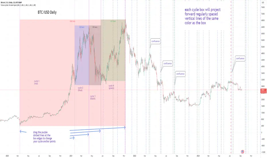
Cycles: 4x dual inputs: Swing / Time Cycles projected forward//Purpose/Premise:
To project forward vertical 'cycle' lines based on user-input anchor points, and to search for confluence.
The idea being that if several well-anchored cycles agree (i.e. we see multiple bunched vertical line confluence in the future), then this may add support to an already existing trade idea, or may indicate an increased likelihood of a shift in direction.
//Usage & notes:
~In the above chart I've anchored to obvious swing lows and swing highs in Btc/Usd from 2020-2022. You could also use fixed time-based cycles from a favored start anchor point. Bars per cycle are printed at the top of each cycle box if your're interested in time cycles. I.e. for 1, 2, 3 month cycles: for BTC you could use 30, 60, 90 bars on daily; for S&P you could use 20, 40, 60 bars on daily.
~On first loading the indicator you will be asked select 'start date', and 'end date' for each of 4 sessions (8x clicks on chart). After this you can easily reset points by clicking the indicator display line three dots>> reset points. Or you can simply drag the vertical box edges (purple lines) to change your cycle anchor points.
~Be sure the start anchor point is before the end anchor point or box/lines won't appear.
~When you drop down to low timeframes you might get bar_index error due to history available: you need then to click the three dots on indicator display line >> reset points >> 8x clicks on the chart.
~Vertical projected lines will match the color of the cycle box they origninate from.
~Lines will project into the future as far as is allowed by tradingview (500 bars max)
//Inputs:
~Time start and end dates for each cycle (change these as described above, or input manually)
~Show/hide each cycle (default is show all 4)
~Formatting options: color of forward projected lines, line width, line style, line / box / text color.
~Box transparancy: Set to 100 to make boxes invisible & declutter the chart. Set to 0 for maximum opacity. Default is 80.
thanks to @Sathyamurthie for his ideas on cycle confluence which caused me to write this.
HK Percentile Interpolation One
This script is designed to execute a trading strategy based on Heikin Ashi candlesticks, moving averages, and percentile levels.
Please note that you should keep your original chart in normal candlestick mode and not switch it to Heikin Ashi mode. The script itself calculates Heikin Ashi values from regular candlesticks. If your chart is already in Heikin Ashi mode, the script would be calculating Heikin Ashi values based on Heikin Ashi values, which would produce incorrect results.
The strategy begins trading from a start date that you can specify by modifying the `startDate` parameter. The format of the date is "YYYY MM DD". So, for example, to start the strategy from January 1, 2022, you would set `startDate = timestamp("2022 01 01")`.
The script uses Heikin Ashi candlesticks, which are plotted in the chart. This approach can be useful for spotting trends and reversals more easily than with regular candlestick charts. This is particularly useful when backtesting in TradingView's "Rewind" mode, as you can see how the Heikin Ashi candles behaved at each step of the strategy.
Buy and sell signals are generated based on two factors:
1. The crossing over or under of the Heikin Ashi close price and the 75th percentile price level.
2. The Heikin Ashi close price being above certain moving averages.
You have the flexibility to adjust several parameters in the script, including:
1. The stop loss and trailing stop percentages (`stopLossPercentage` and `trailStopPercentage`). These parameters allow the strategy to exit trades if the price moves against you by a certain percentage.
2. The lookback period (`lookback`) used to calculate percentile levels. This determines the range of past bars used in the percentile calculation.
3. The lengths of the two moving averages (`yellowLine_length` and `purplLine_length`). These determine how sensitive the moving averages are to recent price changes.
4. The minimum holding period (`holdPeriod`). This sets the minimum number of bars that a trade must be kept open before it can be closed.
Please adjust these parameters according to your trading preferences and risk tolerance. Happy trading!
Pure Morning 2.0 - Candlestick Pattern Doji StrategyThe new "Pure Morning 2.0 - Candlestick Pattern Doji Strategy" is a trend-following, intraday cryptocurrency trading system authored by devil_machine.
The system identifies Doji and Morning Doji Star candlestick formations above the EMA60 as entry points for long trades.
For best results we recommend to use on 15-minute, 30-minute, or 1-hour timeframes, and are ideal for high-volatility markets.
The strategy also utilizes a profit target or trailing stop for exits, with stop loss set at the lowest low of the last 100 candles. The strategy's configuration details, such as Doji tolerance, and exit configurations are adjustable.
In this new version 2.0, we've incorporated a new selectable filter. Since the stop loss is set at the lowest low, this filter ensures that this value isn't too far from the entry price, thereby optimizing the Risk-Reward ratio.
In the specific case of ALPINE, a 9% Take-Profit and and Stop-Loss at Lowest Low of the last 100 candles were set, with an activated trailing-stop percentage, Max Loss Filter is not active.
Name : Pure Morning 2.0 - Candlestick Pattern Doji Strategy
Author : @devil_machine
Category : Trend Follower based on candlestick patterns.
Operating mode : Spot or Futures (only long).
Trades duration : Intraday
Timeframe : 15m, 30m, 1H
Market : Crypto
Suggested usage : Short-term trading, when the market is in trend and it is showing high volatility .
Entry : When a Doji or Morning Doji Star formation occurs above the EMA60.
Exit : Profit target or Trailing stop, Stop loss on the lowest low of the last 100 candles.
Configuration :
- Doji Settings (tolerances) for Entry Condition
- Max Loss Filter (Lowest Low filter)
- Exit Long configuration
- Trailing stop
Backtesting :
⁃ Exchange: BINANCE
⁃ Pair: ALPINEUSDT
⁃ Timeframe: 30m
⁃ Fee: 0.075%
⁃ Slippage: 1
- Initial Capital: 10000 USDT
- Position sizing: 10% of Equity
- Start: 2022-02-28 (Out Of Sample from 2022-12-23)
- Bar magnifier: on
Disclaimer : Risk Management is crucial, so adjust stop loss to your comfort level. A tight stop loss can help minimise potential losses. Use at your own risk.
How you or we can improve? Source code is open so share your ideas!
Leave a comment and smash the boost button!
Thanks for your attention, happy to support the TradingView community.

Strategy Template + Performance & Returns table + ExtrasA script I've been working on since summer 2022. A template for any strategy so you just have to write or paste the code and go straight into risk management settings
Features:
>Signal only Longs/only Shorts/Both
>Leverage system
>Proper fees calculation (even with leverage on)
>Different Stop Loss systems: Simple percentage, 4 different "move to Break Even" systems and Scaling SL after each TP order (read the disclaimer at the bottom regarding this and the TV % profitable metric)
>2 Take Profit systems: Simple percentages, or Risk/reward ratios based on SL level
>Additional option on TP so last one "rides free" until closure of position or Stoploss is hit (for more than 1 orders)
>Up to 5 TP orders
>Show or hide SL/TP levels on demand
>2 date filters. Manual filter is nothing new, enter two dates/hours and filter will turn on. BUT automatic filter is another thing (thanks to user @bfr_ for his help in codingthis feature)
>AUTOMATIC DATE FILTER. Allows you to split all historical data on the chart in X periods, then choose the range of periods used. Up to 10 but that can be changed, instructions included. Useful for WalkForward simulations, haven't seen a script in TradingView that allows you to do this and test your strategy on "unseen data" automatically
EXTRA SETTINGS
Besides, some additions I like to add to my codes:
>Returns table for monthly and weekly performance. Requires recalculation on every tick. This is a modified version of @QuantNomad's work. May add lower TF options later on
>Volume Based S/R system. Original work from @shtcoinr
>One feature that was made by me, the "portfolio table". Yields info and metrics of your strategy, current position and balance. You're able to turn it off and change its size
Should anyone find an error, or have any idea on how to improve this code, please contact me. Future updates could come, stay tuned
DISCLAIMER:
In order to have accurate StopLoss hit, I had to change the previous system, which was a "close position on candle close" instead at actual stoploss level. It was fixed, but resulted on inflation of the number of trading orders, thus reducing the percent profitable and making it strongly biased and unreal. Keep that in mind, that "real" profitability could be 2x or 3x the metric TradingView says. If your strategy has a really high trading frequency, resulting in 3000+ orders, might be a problem. Try to make use of the automatic/manual date filter as workaround, I have no means of changing this, seems it is not a bug but an intended design of the PineScript Code

Multi-Asset Month/Month % change 10yr Averages10 Year Averages of Month-on-Month % change: Shows current asset, and 3x user input assets
-For comparing seasonal tendencies among different assets.
-Choose from a variety of monthly average measures as source: sma(close, length), sma(ohlc4, length); as well as sma's of vwap, vwma, volume, volatility. (sma = simple moving average).
-Averages based on month cf previous month: i.e. Feb % = Feb compared to Jan; Jan % = Jan compared to prev year's Dec. Average of the last 10yrs of these values is the printed value.
-Plot on current year (2023), or previous year (2022). If Plotting on current year, and a month of year has not yet occured, a 9yr average will be printed.
/// notes ///
-daily bars in month is a global setting; so choose assets which have similar trading days per month. i.e. Crypto: length = 30 (days per month); Stocks/FX/Indices: length = 21 (days per month).
-only plots on Daily timeframe.
10yr Avgs; Plotting with Year = 2022; using sma(close, 21) as source for average M/M change

Weis V5 zigzag jayySomehow, I deleted version 5 of the zigzag script. Same name. I have added some older notes describing how the Weis Wave works.
I have also changed the date restriction that stopped the script from working after Dec 31, 2022.
What you see here is the Weis zigzag wave plotted directly on the price chart. This script is the companion to the Weis cumulative wave volume script.
What is a Weis wave? David Weis has been recognized as a Wyckoff method analyst he has written two books one of which, Trades About to Happen, describes the evolution of the now-popular Weis wave. The method employed by Weis is to identify waves of price action and to compare the strength of the waves on characteristics of wave strength. Chief among the characteristics of strength is the cumulative volume of the wave. There are other markers that Weis uses as well for example how the actual price difference between the start of the Weis wave from start to finish. Weis also uses time, particularly when using a Renko chart
David Weis did a futures io video which is a popular source of information about his method. (Search David Weis and futures.io. I strongly suggest you also read “Trades About to Happen” by David Weis.
This will get you up and running more quickly when studying charts. However, you should choose the Traditional method to be true to David Weis technique as described in his book "Trades About to Happen" and in the Futures IO Webcast featuring David Weis
. The Weis pip zigzag wave shows how far in terms of bar close price a Weis wave has traveled through the duration of a Weis wave. The Weis zigzag wave is used in combination with the Weis cumulative volume wave. The two waves should be set to the same "wave size".
To use this script, you must set the wave size: Using the traditional Weis method simply enter the desired wave size in the box "How should wave size be calculated", in this example I am using a traditional wave size of .25. Each wave for each security and each timeframe requires its own wave size. Although not the traditional method devised by David Weis a more automatic way to set wave size would be to use Average True Range (ATR). Using ATR is not the true Weis method but it does give you similar waves and, importantly, without the hassle described above. Once the Weis wave size is set then the zigzag wave will be shown with volume. Because Weis used the closing price of a wave to define waves a line Bar highs and bar lows are not captured by the Weis Wave. The default script setting is now cumulative volume waves using an ATR of 7 and a multiplication factor of .5.
To display volume in a way that does not crowd out neighbouring volumes Weis displayed volume as a maximum of 3 digits (usually). Consider two Weis Wave volumes 176,895,570 and 2,654,763,889. To display wave volume as three digits it is necessary to take a number such as 176,895,570 and truncate it. 176,895,570 can be represented as 177 X 10 to the power of 6. The number displayed must also be relative to other numbers in the field. If the highest volume on the page is: 2,654,763,889 and with only three numbers available to display the result the value shown must be 265 (265 X 10 to the power of 7). Since 176,895,570 is an order of magnitude smaller than 2,654,763,889 therefore 175,895,570 must be shown as 18 instead of 177. In this way, the relative magnitudes of the two volumes can be understood. All numbers in the field of view must be truncated by the same order of magnitude to make the relative volumes understandable. The script attempts to calculate the order of magnitude value automatically. If you see a red number in the field of view it means the script has failed to do the calculation automatically and you should use the manual method – use the dialogue box “Calculate truncated wave value automatically or manually”. Scroll down from the automatic method and select manual. Once "manual" is selected the values displayed become the power values or multipliers for each wave.
Using the manual method you will select a “Multiplier” in the next dialogue box. Scan the field and select the largest value in the field of view (visible chart) is the multiplier of interest. If you select a lower number than the maximum value will see at least one red “up”. If you are too high you will see at least one red “down”. Scroll in the direction recommended or the values on the screen will be totally incorrect. With volume truncated to the highest order values, the eye can quickly get a feel for relative volumes. It also reduces the crowding and overlapping of values on the screen. You can opt to show the full volume to help get a sense of the magnitude of the true volumes.
How does the script determine if a Weis wave is continuing to grow or not?
The script evaluates the closing price of each new bar relative to the "Weis wave size". Suppose the current bar closes at a new low close, within the current down wave, at $30.00. If the Weis wave size is $0.10 then the algorithm will remember the $30.00 close and compare it to the close of the next bar. If the bar close price does not close equal to or lower than $30.00 or close equal to or higher than $30.10 then the wave is still a down wave with a current low of $30.00. This is true even if the bar low is less than $30.00 or the bar high is greater than 30.10 – only the bar’s closing price matters. If a bar's closing price climbs back up to a close of $30.11 then because the closing price has moved more than $0.10 (the Weis wave size) then that is a wave reversal with a new up-trending wave. In the above example if there was currently a downward trending wave and the bar closes were as follows $30.00, $30.09, $30.01, $30.05, $30.10 The wave direction would continue to stay downward trending until the close of $30.10 was achieved. As such $30.00 would be the low and the following closes $30.09, $30.01, $30.05 would be allocated to the new upward-trending wave. If however There was a series of bar closes like this $30.00, $30.09, $30.01, $30.05, $29.99 since none of the closes was equal to above the 10-cent reversal target of $30.10 but instead, a new Weis wave low was achieved ($29.99). As such the closes of $30.09, $30.01, $30.05 would all be attributed to the continued down-trending wave with a current low of $29.99, even though the closing price for the interim bars was above $30.00. Now that the Weis Wave low is now 429.99 then, in order to reverse this continued downtrend price will need to close at or above $30.09 on subsequent bar closes assuming now new low bar close is achieved. With large wave sizes, wave direction can be in limbo for many bars before a close either renews wave direction or reverses it and confirms wave direction as either a reversal or a continuation. On the zig-zag, a wave line and its volume will not be "printed" until a wave reversal is confirmed.
The wave attribution is similar when using other methods to define wave size. If ATR is used for wave size instead of a traditional wave constant size such as $0.10 or $2 or 2000 pips or ... then the wave size is calculated based on current ATR instead of the Weis wave constant (Traditional selected value).
I have the option to display pseudo-Ord volume. In truth, Ord used more traditional zig-zag pivots of bar highs and lows. Waves using closes as pivots can have some significant differences. This difference can be lessened by using smaller time frames and larger wave sizes.
There are other options such to display the delta price or pip size of a Weis Wave, the number of bars in a wave, and a few other options.

Moving Average Cross and RSIThis is the updated version of the MAC cross Short/ Long indicator i had posted earlier in 2022.
This script includes a RSI and EMA of the RSI with fixed OB and OS Levels.
The purpose is to refine the amount of trades taken from the moving average cross on the 30 minute timeframe.
In the overlay, the red and green dots indicate weather the moving cross is a long or a short signal.
The theory when back tested is:
When the short signal is given, the EMA must be below 30 to enter a short.
When the long signal is given, the EMA must be above 64 to enter a long, anything in between is a false signal.
Only the first dot is meant to be a long or a short signal, not meant to be interpreted as being consecutive.
The data window is meant to be built in a way to easily set up indicators or strategies using Tradelab.ai software.

DR/IDR Candles [LuxAlgo]This indicator displays defining ranges (DR) and implied defining ranges (IDR) constructed from two user set sessions (RDR/ODR) as graphical candles on the chart. The script introduces additional graphical elements to the original DR/IDR concept and as such can be thought as a graphical method in addition to a technical indicator.
Additionally, this script can display various Fibonacci retracements from the constructed DR/IDR if enabled within the settings.
Settings
Regular Session: Enable/disable regular session's DR/IDR alongside setting the session time. By default, 09:30 - 10:30 am.
Overnight Session: Enable/disable overnight session's DR/IDR alongside setting the session time. By default, 03:00 - 04:00 am.
UTC Offset: UTC offset for the time zone, by default -5 (EST)
Retracements
Reverse: Inverts source range upper/lower value for constructing the retracements.
From: Source range used to construct the retracements, by default DR is used.
By default, the 0.5 retracement (average line) is displayed.
Usage
The used sessions are highlighted by a gray background. DRs are highlighted by dashed lines while IDRs are highlighted by solid ones. The maximum/minimum price between each user set session is highlighted by solid wicks.
The color of the DRs/IDRs/wicks are determined by the price position relative to the DR; if price is above the DR maximum, then a blue color is used. If price is below, then an orange color is used, and if price is within the DR range, then a gray color is used.
Additionally, the area of the DR range is used to highlight the number of time price is located within the DR, with a longer background highlighting a higher number of occurrences. This can help highlight if the DR levels were potentially useful as support/resistance.
When price is outside the IDR range, the area between the price and IDR is highlighted, in blue if price is above the IDR, and orange if it is under.
The original author of the DR/IDR concept describes 3 rules using the price position relative to the DR/IDR levels:
1.) If price on the 5-minute timeframe closes above the DR high after 10:30 AM or 04:00 AM then the DR low will likely be the low of the trading session.
2.) If price on the 5-minute timeframe closes below the DR low after 10:30 AM or 04:00 AM then the DR high will likely be the high of the trading session.
3.) If price closes above the IDR high after 10:30 AM or 04:00 AM it is an early indication that the low of the DR will be the low of the day and vice versa.
We can see that the above rules are cases of conditional probabilities.
There is no significant data supporting or regarding any statistical probability of the above rules to be true, which are more than uncertain given the stochastic nature of prices. The lack of precision of these rules is also a concern (time zone dependance, applicable markets, etc...).
Credits
Credits to trader TheMas7er who originally created the DR/IDR concept in November of 2022. This script was derived from his proposed session times & rules for trading.