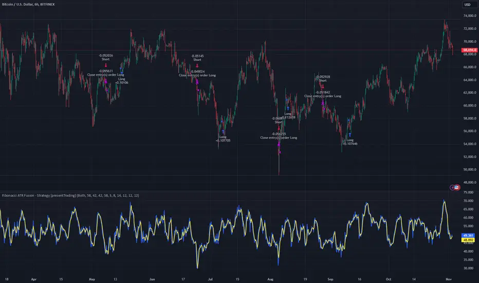
Fibonacci ATR Fusion - Strategy [presentTrading]Open-script again! This time is also an ATR-related strategy. Enjoy! :)
If you have any questions, let me know, and I'll help make this as effective as possible.
█ Introduction and How It Is Different
The Fibonacci ATR Fusion Strategy is an advanced trading approach that uniquely integrates Fibonacci-based weighted averages with the Average True Range (ATR) to identify and capitalize on significant market trends.
Unlike traditional strategies that rely on single indicators or static parameters, this method combines multiple timeframes and dynamic volatility measurements to enhance precision and adaptability. Additionally, it features a 4-step Take Profit (TP) mechanism, allowing for systematic profit-taking at various levels, which optimizes both risk management and return potential in long and short market positions.
BTCUSD 6hr Performance
█ Strategy, How It Works: Detailed Explanation
The Fibonacci ATR Fusion Strategy utilizes a combination of technical indicators and weighted averages to determine optimal entry and exit points. Below is a breakdown of its key components and operational logic.
🔶 1. Enhanced True Range Calculation
The strategy begins by calculating the True Range (TR) to measure market volatility accurately.
TR = max(High - Low, abs(High - Previous Close), abs(Low - Previous Close))
High and Low: Highest and lowest prices of the current trading period.
Previous Close: Closing price of the preceding trading period.
max: Selects the largest value among the three calculations to account for gaps and limit movements.
🔶 2. Buying Pressure (BP) Calculation
Buying Pressure (BP) quantifies the extent to which buyers are driving the price upwards within a period.
BP = Close - True Low
Close: Current period's closing price.
True Low: The lower boundary determined in the True Range calculation.
🔶 3. Ratio Calculation for Different Periods
To assess the strength of buying pressure relative to volatility, the strategy calculates a ratio over various Fibonacci-based timeframes.
Ratio = 100 * (Sum of BP over n periods) / (Sum of TR over n periods)
n: Length of the period (e.g., 8, 13, 21, 34, 55).
Sum of BP: Cumulative Buying Pressure over n periods.
Sum of TR: Cumulative True Range over n periods.
This ratio normalizes buying pressure, making it comparable across different timeframes.
🔶 4. Weighted Average Calculation
The strategy employs a weighted average of ratios from multiple Fibonacci-based periods to smooth out signals and enhance trend detection.
Weighted Avg = (w1 * Ratio_p1 + w2 * Ratio_p2 + w3 * Ratio_p3 + w4 * Ratio_p4 + Ratio_p5) / (w1 + w2 + w3 + w4 + 1)
w1, w2, w3, w4: Weights assigned to each ratio period.
Ratio_p1 to Ratio_p5: Ratios calculated for periods p1 to p5 (e.g., 8, 13, 21, 34, 55).
This weighted approach emphasizes shorter periods more heavily, capturing recent market dynamics while still considering longer-term trends.
🔶 5. Simple Moving Average (SMA) of Weighted Average
To further smooth the weighted average and reduce noise, a Simple Moving Average (SMA) is applied.
Weighted Avg SMA = SMA(Weighted Avg, m)
- m: SMA period (e.g., 3).
This smoothed line serves as the primary signal generator for trade entries and exits.
🔶 6. Trading Condition Thresholds
The strategy defines specific threshold values to determine optimal entry and exit points based on crossovers and crossunders of the SMA.
Long Condition = Crossover(Weighted Avg SMA, Long Entry Threshold)
Short Condition = Crossunder(Weighted Avg SMA, Short Entry Threshold)
Long Exit = Crossunder(Weighted Avg SMA, Long Exit Threshold)
Short Exit = Crossover(Weighted Avg SMA, Short Exit Threshold)
Long Entry Threshold (T_LE): Level at which a long position is triggered.
Short Entry Threshold (T_SE): Level at which a short position is triggered.
Long Exit Threshold (T_LX): Level at which a long position is exited.
Short Exit Threshold (T_SX): Level at which a short position is exited.
These conditions ensure that trades are only executed when clear trends are identified, enhancing the strategy's reliability.
Previous local performance
🔶 7. ATR-Based Take Profit Mechanism
When enabled, the strategy employs a 4-step Take Profit system to systematically secure profits as the trade moves in the desired direction.
TP Price_1 Long = Entry Price + (TP1ATR * ATR Value)
TP Price_2 Long = Entry Price + (TP2ATR * ATR Value)
TP Price_3 Long = Entry Price + (TP3ATR * ATR Value)
TP Price_1 Short = Entry Price - (TP1ATR * ATR Value)
TP Price_2 Short = Entry Price - (TP2ATR * ATR Value)
TP Price_3 Short = Entry Price - (TP3ATR * ATR Value)
- ATR Value: Calculated using ATR over a specified period (e.g., 14).
- TPxATR: User-defined multipliers for each take profit level.
- TPx_percent: Percentage of the position to exit at each TP level.
This multi-tiered exit strategy allows for partial position closures, optimizing profit capture while maintaining exposure to potential further gains.
█ Trade Direction
The Fibonacci ATR Fusion Strategy is designed to operate in both long and short market conditions, providing flexibility to traders in varying market environments.
Long Trades: Initiated when the SMA of the weighted average crosses above the Long Entry Threshold (T_LE), indicating strong upward momentum.
Short Trades: Initiated when the SMA of the weighted average crosses below the Short Entry Threshold (T_SE), signaling robust downward momentum.
Additionally, the strategy can be configured to trade exclusively in one direction—Long, Short, or Both—based on the trader’s preference and market analysis.
█ Usage
Implementing the Fibonacci ATR Fusion Strategy involves several steps to ensure it aligns with your trading objectives and market conditions.
1. Configure Strategy Parameters:
- Trading Direction: Choose between Long, Short, or Both based on your market outlook.
- Trading Condition Thresholds: Set the Long Entry, Short Entry, Long Exit, and Short Exit thresholds to define when to enter and exit trades.
2. Set Take Profit Levels (if enabled):
- ATR Multipliers: Define how many ATRs away from the entry price each take profit level is set.
- Take Profit Percentages: Allocate what percentage of the position to close at each TP level.
3. Apply to Desired Chart:
- Add the strategy to the chart of the asset you wish to trade.
- Observe the plotted Fibonacci ATR and SMA Fibonacci ATR indicators for visual confirmation.
4. Monitor and Adjust:
- Regularly review the strategy’s performance through backtesting.
- Adjust the input parameters based on historical performance and changing market dynamics.
5. Risk Management:
- Ensure that the sum of take profit percentages does not exceed 100% to avoid over-closing positions.
- Utilize the ATR-based TP levels to adapt to varying market volatilities, maintaining a balanced risk-reward ratio.
█ Default Settings
Understanding the default settings is crucial for optimizing the Fibonacci ATR Fusion Strategy's performance. Here's a precise and simple overview of the key parameters and their effects:
🔶 Key Parameters and Their Effects
1. Trading Direction (`tradingDirection`)
- Default: Both
- Effect: Determines whether the strategy takes both long and short positions or restricts to one direction. Selecting Both allows maximum flexibility, while Long or Short can be used for directional bias.
2. Trading Condition Thresholds
Long Entry (long_entry_threshold = 58.0): Higher values reduce false positives but may miss trades.
Short Entry (short_entry_threshold = 42.0): Lower values capture early short trends but may increase false signals.
Long Exit (long_exit_threshold = 42.0): Exits long positions early, securing profits but potentially cutting trends short.
Short Exit (short_exit_threshold = 58.0): Delays short exits to capture favorable movements, avoiding premature exits.
3. Take Profit Configuration (`useTakeProfit` = false)
- Effect: When enabled, the strategy employs a 4-step TP mechanism to secure profits at multiple levels. By default, it is disabled to allow users to opt-in based on their trading style.
4. ATR-Based Take Profit Multipliers
TP1 (tp1ATR = 3.0): Sets the first TP at 3 ATRs for initial profit capture.
TP2 (tp2ATR = 8.0): Targets larger trends, though less likely to be reached.
TP3 (tp3ATR = 14.0): Optimizes for extreme price moves, seldom triggered.
5. Take Profit Percentages
TP Level 1 (tp1_percent = 12%): Secures 12% at the first TP.
TP Level 2 (tp2_percent = 12%): Exits another 12% at the second TP.
TP Level 3 (tp3_percent = 12%): Closes an additional 12% at the third TP.
6. Weighted Average Parameters
Ratio Periods: Fibonacci-based intervals (8, 13, 21, 34, 55) balance responsiveness.
Weights: Emphasizes recent data for timely responses to market trends.
SMA Period (weighted_avg_sma_period = 3): Smoothens data with minimal lag, balancing noise reduction and responsiveness.
7. ATR Period (`atrPeriod` = 14)
Effect: Sets the ATR calculation length, impacting TP sensitivity to volatility.
🔶 Impact on Performance
- Sensitivity and Responsiveness:
- Shorter Ratio Periods and Higher Weights: Make the weighted average more responsive to recent price changes, allowing quicker trade entries and exits but increasing the likelihood of false signals.
- Longer Ratio Periods and Lower Weights: Provide smoother signals with fewer false positives but may delay trade entries, potentially missing out on significant price moves.
- Profit Taking:
- ATR Multipliers: Higher multipliers set take profit levels further away, targeting larger price movements but reducing the probability of reaching these levels.
- Fixed Percentages: Allocating equal percentages at each TP level ensures consistent profit realization and risk management, preventing overexposure.
- Trade Direction Control:
- Selecting Specific Directions: Restricting trades to Long or Short can align the strategy with market trends or personal biases, potentially enhancing performance in trending markets.
- Risk Management:
- Take Profit Percentages: Dividing the position into smaller percentages at multiple TP levels helps lock in profits progressively, reducing risk and allowing the remaining position to ride further trends.
- Market Adaptability:
- Weighted Averages and ATR: By combining multiple timeframes and adjusting to volatility, the strategy adapts to different market conditions, maintaining effectiveness across various asset classes and timeframes.
---
If you want to know more about ATR, can also check "SuperATR 7-Step Profit".
Enjoy trading.
Wyszukaj w skryptach "细算江西救护车家长倒赚了四万三+-医疗花费13万(家长视频)++医保报"
Universal Ratio Trend Matrix [InvestorUnknown]The Universal Ratio Trend Matrix is designed for trend analysis on asset/asset ratios, supporting up to 40 different assets. Its primary purpose is to help identify which assets are outperforming others within a selection, providing a broad overview of market trends through a matrix of ratios. The indicator automatically expands the matrix based on the number of assets chosen, simplifying the process of comparing multiple assets in terms of performance.
Key features include the ability to choose from a narrow selection of indicators to perform the ratio trend analysis, allowing users to apply well-defined metrics to their comparison.
Drawback: Due to the computational intensity involved in calculating ratios across many assets, the indicator has a limitation related to loading speed. TradingView has time limits for calculations, and for users on the basic (free) plan, this could result in frequent errors due to exceeded time limits. To use the indicator effectively, users with any paid plans should run it on timeframes higher than 8h (the lowest timeframe on which it managed to load with 40 assets), as lower timeframes may not reliably load.
Indicators:
RSI_raw: Simple function to calculate the Relative Strength Index (RSI) of a source (asset price).
RSI_sma: Calculates RSI followed by a Simple Moving Average (SMA).
RSI_ema: Calculates RSI followed by an Exponential Moving Average (EMA).
CCI: Calculates the Commodity Channel Index (CCI).
Fisher: Implements the Fisher Transform to normalize prices.
Utility Functions:
f_remove_exchange_name: Strips the exchange name from asset tickers (e.g., "INDEX:BTCUSD" to "BTCUSD").
f_remove_exchange_name(simple string name) =>
string parts = str.split(name, ":")
string result = array.size(parts) > 1 ? array.get(parts, 1) : name
result
f_get_price: Retrieves the closing price of a given asset ticker using request.security().
f_constant_src: Checks if the source data is constant by comparing multiple consecutive values.
Inputs:
General settings allow users to select the number of tickers for analysis (used_assets) and choose the trend indicator (RSI, CCI, Fisher, etc.).
Table settings customize how trend scores are displayed in terms of text size, header visibility, highlighting options, and top-performing asset identification.
The script includes inputs for up to 40 assets, allowing the user to select various cryptocurrencies (e.g., BTCUSD, ETHUSD, SOLUSD) or other assets for trend analysis.
Price Arrays:
Price values for each asset are stored in variables (price_a1 to price_a40) initialized as na. These prices are updated only for the number of assets specified by the user (used_assets).
Trend scores for each asset are stored in separate arrays
// declare price variables as "na"
var float price_a1 = na, var float price_a2 = na, var float price_a3 = na, var float price_a4 = na, var float price_a5 = na
var float price_a6 = na, var float price_a7 = na, var float price_a8 = na, var float price_a9 = na, var float price_a10 = na
var float price_a11 = na, var float price_a12 = na, var float price_a13 = na, var float price_a14 = na, var float price_a15 = na
var float price_a16 = na, var float price_a17 = na, var float price_a18 = na, var float price_a19 = na, var float price_a20 = na
var float price_a21 = na, var float price_a22 = na, var float price_a23 = na, var float price_a24 = na, var float price_a25 = na
var float price_a26 = na, var float price_a27 = na, var float price_a28 = na, var float price_a29 = na, var float price_a30 = na
var float price_a31 = na, var float price_a32 = na, var float price_a33 = na, var float price_a34 = na, var float price_a35 = na
var float price_a36 = na, var float price_a37 = na, var float price_a38 = na, var float price_a39 = na, var float price_a40 = na
// create "empty" arrays to store trend scores
var a1_array = array.new_int(40, 0), var a2_array = array.new_int(40, 0), var a3_array = array.new_int(40, 0), var a4_array = array.new_int(40, 0)
var a5_array = array.new_int(40, 0), var a6_array = array.new_int(40, 0), var a7_array = array.new_int(40, 0), var a8_array = array.new_int(40, 0)
var a9_array = array.new_int(40, 0), var a10_array = array.new_int(40, 0), var a11_array = array.new_int(40, 0), var a12_array = array.new_int(40, 0)
var a13_array = array.new_int(40, 0), var a14_array = array.new_int(40, 0), var a15_array = array.new_int(40, 0), var a16_array = array.new_int(40, 0)
var a17_array = array.new_int(40, 0), var a18_array = array.new_int(40, 0), var a19_array = array.new_int(40, 0), var a20_array = array.new_int(40, 0)
var a21_array = array.new_int(40, 0), var a22_array = array.new_int(40, 0), var a23_array = array.new_int(40, 0), var a24_array = array.new_int(40, 0)
var a25_array = array.new_int(40, 0), var a26_array = array.new_int(40, 0), var a27_array = array.new_int(40, 0), var a28_array = array.new_int(40, 0)
var a29_array = array.new_int(40, 0), var a30_array = array.new_int(40, 0), var a31_array = array.new_int(40, 0), var a32_array = array.new_int(40, 0)
var a33_array = array.new_int(40, 0), var a34_array = array.new_int(40, 0), var a35_array = array.new_int(40, 0), var a36_array = array.new_int(40, 0)
var a37_array = array.new_int(40, 0), var a38_array = array.new_int(40, 0), var a39_array = array.new_int(40, 0), var a40_array = array.new_int(40, 0)
f_get_price(simple string ticker) =>
request.security(ticker, "", close)
// Prices for each USED asset
f_get_asset_price(asset_number, ticker) =>
if (used_assets >= asset_number)
f_get_price(ticker)
else
na
// overwrite empty variables with the prices if "used_assets" is greater or equal to the asset number
if barstate.isconfirmed // use barstate.isconfirmed to avoid "na prices" and calculation errors that result in empty cells in the table
price_a1 := f_get_asset_price(1, asset1), price_a2 := f_get_asset_price(2, asset2), price_a3 := f_get_asset_price(3, asset3), price_a4 := f_get_asset_price(4, asset4)
price_a5 := f_get_asset_price(5, asset5), price_a6 := f_get_asset_price(6, asset6), price_a7 := f_get_asset_price(7, asset7), price_a8 := f_get_asset_price(8, asset8)
price_a9 := f_get_asset_price(9, asset9), price_a10 := f_get_asset_price(10, asset10), price_a11 := f_get_asset_price(11, asset11), price_a12 := f_get_asset_price(12, asset12)
price_a13 := f_get_asset_price(13, asset13), price_a14 := f_get_asset_price(14, asset14), price_a15 := f_get_asset_price(15, asset15), price_a16 := f_get_asset_price(16, asset16)
price_a17 := f_get_asset_price(17, asset17), price_a18 := f_get_asset_price(18, asset18), price_a19 := f_get_asset_price(19, asset19), price_a20 := f_get_asset_price(20, asset20)
price_a21 := f_get_asset_price(21, asset21), price_a22 := f_get_asset_price(22, asset22), price_a23 := f_get_asset_price(23, asset23), price_a24 := f_get_asset_price(24, asset24)
price_a25 := f_get_asset_price(25, asset25), price_a26 := f_get_asset_price(26, asset26), price_a27 := f_get_asset_price(27, asset27), price_a28 := f_get_asset_price(28, asset28)
price_a29 := f_get_asset_price(29, asset29), price_a30 := f_get_asset_price(30, asset30), price_a31 := f_get_asset_price(31, asset31), price_a32 := f_get_asset_price(32, asset32)
price_a33 := f_get_asset_price(33, asset33), price_a34 := f_get_asset_price(34, asset34), price_a35 := f_get_asset_price(35, asset35), price_a36 := f_get_asset_price(36, asset36)
price_a37 := f_get_asset_price(37, asset37), price_a38 := f_get_asset_price(38, asset38), price_a39 := f_get_asset_price(39, asset39), price_a40 := f_get_asset_price(40, asset40)
Universal Indicator Calculation (f_calc_score):
This function allows switching between different trend indicators (RSI, CCI, Fisher) for flexibility.
It uses a switch-case structure to calculate the indicator score, where a positive trend is denoted by 1 and a negative trend by 0. Each indicator has its own logic to determine whether the asset is trending up or down.
// use switch to allow "universality" in indicator selection
f_calc_score(source, trend_indicator, int_1, int_2) =>
int score = na
if (not f_constant_src(source)) and source > 0.0 // Skip if you are using the same assets for ratio (for example BTC/BTC)
x = switch trend_indicator
"RSI (Raw)" => RSI_raw(source, int_1)
"RSI (SMA)" => RSI_sma(source, int_1, int_2)
"RSI (EMA)" => RSI_ema(source, int_1, int_2)
"CCI" => CCI(source, int_1)
"Fisher" => Fisher(source, int_1)
y = switch trend_indicator
"RSI (Raw)" => x > 50 ? 1 : 0
"RSI (SMA)" => x > 50 ? 1 : 0
"RSI (EMA)" => x > 50 ? 1 : 0
"CCI" => x > 0 ? 1 : 0
"Fisher" => x > x ? 1 : 0
score := y
else
score := 0
score
Array Setting Function (f_array_set):
This function populates an array with scores calculated for each asset based on a base price (p_base) divided by the prices of the individual assets.
It processes multiple assets (up to 40), calling the f_calc_score function for each.
// function to set values into the arrays
f_array_set(a_array, p_base) =>
array.set(a_array, 0, f_calc_score(p_base / price_a1, trend_indicator, int_1, int_2))
array.set(a_array, 1, f_calc_score(p_base / price_a2, trend_indicator, int_1, int_2))
array.set(a_array, 2, f_calc_score(p_base / price_a3, trend_indicator, int_1, int_2))
array.set(a_array, 3, f_calc_score(p_base / price_a4, trend_indicator, int_1, int_2))
array.set(a_array, 4, f_calc_score(p_base / price_a5, trend_indicator, int_1, int_2))
array.set(a_array, 5, f_calc_score(p_base / price_a6, trend_indicator, int_1, int_2))
array.set(a_array, 6, f_calc_score(p_base / price_a7, trend_indicator, int_1, int_2))
array.set(a_array, 7, f_calc_score(p_base / price_a8, trend_indicator, int_1, int_2))
array.set(a_array, 8, f_calc_score(p_base / price_a9, trend_indicator, int_1, int_2))
array.set(a_array, 9, f_calc_score(p_base / price_a10, trend_indicator, int_1, int_2))
array.set(a_array, 10, f_calc_score(p_base / price_a11, trend_indicator, int_1, int_2))
array.set(a_array, 11, f_calc_score(p_base / price_a12, trend_indicator, int_1, int_2))
array.set(a_array, 12, f_calc_score(p_base / price_a13, trend_indicator, int_1, int_2))
array.set(a_array, 13, f_calc_score(p_base / price_a14, trend_indicator, int_1, int_2))
array.set(a_array, 14, f_calc_score(p_base / price_a15, trend_indicator, int_1, int_2))
array.set(a_array, 15, f_calc_score(p_base / price_a16, trend_indicator, int_1, int_2))
array.set(a_array, 16, f_calc_score(p_base / price_a17, trend_indicator, int_1, int_2))
array.set(a_array, 17, f_calc_score(p_base / price_a18, trend_indicator, int_1, int_2))
array.set(a_array, 18, f_calc_score(p_base / price_a19, trend_indicator, int_1, int_2))
array.set(a_array, 19, f_calc_score(p_base / price_a20, trend_indicator, int_1, int_2))
array.set(a_array, 20, f_calc_score(p_base / price_a21, trend_indicator, int_1, int_2))
array.set(a_array, 21, f_calc_score(p_base / price_a22, trend_indicator, int_1, int_2))
array.set(a_array, 22, f_calc_score(p_base / price_a23, trend_indicator, int_1, int_2))
array.set(a_array, 23, f_calc_score(p_base / price_a24, trend_indicator, int_1, int_2))
array.set(a_array, 24, f_calc_score(p_base / price_a25, trend_indicator, int_1, int_2))
array.set(a_array, 25, f_calc_score(p_base / price_a26, trend_indicator, int_1, int_2))
array.set(a_array, 26, f_calc_score(p_base / price_a27, trend_indicator, int_1, int_2))
array.set(a_array, 27, f_calc_score(p_base / price_a28, trend_indicator, int_1, int_2))
array.set(a_array, 28, f_calc_score(p_base / price_a29, trend_indicator, int_1, int_2))
array.set(a_array, 29, f_calc_score(p_base / price_a30, trend_indicator, int_1, int_2))
array.set(a_array, 30, f_calc_score(p_base / price_a31, trend_indicator, int_1, int_2))
array.set(a_array, 31, f_calc_score(p_base / price_a32, trend_indicator, int_1, int_2))
array.set(a_array, 32, f_calc_score(p_base / price_a33, trend_indicator, int_1, int_2))
array.set(a_array, 33, f_calc_score(p_base / price_a34, trend_indicator, int_1, int_2))
array.set(a_array, 34, f_calc_score(p_base / price_a35, trend_indicator, int_1, int_2))
array.set(a_array, 35, f_calc_score(p_base / price_a36, trend_indicator, int_1, int_2))
array.set(a_array, 36, f_calc_score(p_base / price_a37, trend_indicator, int_1, int_2))
array.set(a_array, 37, f_calc_score(p_base / price_a38, trend_indicator, int_1, int_2))
array.set(a_array, 38, f_calc_score(p_base / price_a39, trend_indicator, int_1, int_2))
array.set(a_array, 39, f_calc_score(p_base / price_a40, trend_indicator, int_1, int_2))
a_array
Conditional Array Setting (f_arrayset):
This function checks if the number of used assets is greater than or equal to a specified number before populating the arrays.
// only set values into arrays for USED assets
f_arrayset(asset_number, a_array, p_base) =>
if (used_assets >= asset_number)
f_array_set(a_array, p_base)
else
na
Main Logic
The main logic initializes arrays to store scores for each asset. Each array corresponds to one asset's performance score.
Setting Trend Values: The code calls f_arrayset for each asset, populating the respective arrays with calculated scores based on the asset prices.
Combining Arrays: A combined_array is created to hold all the scores from individual asset arrays. This array facilitates further analysis, allowing for an overview of the performance scores of all assets at once.
// create a combined array (work-around since pinescript doesn't support having array of arrays)
var combined_array = array.new_int(40 * 40, 0)
if barstate.islast
for i = 0 to 39
array.set(combined_array, i, array.get(a1_array, i))
array.set(combined_array, i + (40 * 1), array.get(a2_array, i))
array.set(combined_array, i + (40 * 2), array.get(a3_array, i))
array.set(combined_array, i + (40 * 3), array.get(a4_array, i))
array.set(combined_array, i + (40 * 4), array.get(a5_array, i))
array.set(combined_array, i + (40 * 5), array.get(a6_array, i))
array.set(combined_array, i + (40 * 6), array.get(a7_array, i))
array.set(combined_array, i + (40 * 7), array.get(a8_array, i))
array.set(combined_array, i + (40 * 8), array.get(a9_array, i))
array.set(combined_array, i + (40 * 9), array.get(a10_array, i))
array.set(combined_array, i + (40 * 10), array.get(a11_array, i))
array.set(combined_array, i + (40 * 11), array.get(a12_array, i))
array.set(combined_array, i + (40 * 12), array.get(a13_array, i))
array.set(combined_array, i + (40 * 13), array.get(a14_array, i))
array.set(combined_array, i + (40 * 14), array.get(a15_array, i))
array.set(combined_array, i + (40 * 15), array.get(a16_array, i))
array.set(combined_array, i + (40 * 16), array.get(a17_array, i))
array.set(combined_array, i + (40 * 17), array.get(a18_array, i))
array.set(combined_array, i + (40 * 18), array.get(a19_array, i))
array.set(combined_array, i + (40 * 19), array.get(a20_array, i))
array.set(combined_array, i + (40 * 20), array.get(a21_array, i))
array.set(combined_array, i + (40 * 21), array.get(a22_array, i))
array.set(combined_array, i + (40 * 22), array.get(a23_array, i))
array.set(combined_array, i + (40 * 23), array.get(a24_array, i))
array.set(combined_array, i + (40 * 24), array.get(a25_array, i))
array.set(combined_array, i + (40 * 25), array.get(a26_array, i))
array.set(combined_array, i + (40 * 26), array.get(a27_array, i))
array.set(combined_array, i + (40 * 27), array.get(a28_array, i))
array.set(combined_array, i + (40 * 28), array.get(a29_array, i))
array.set(combined_array, i + (40 * 29), array.get(a30_array, i))
array.set(combined_array, i + (40 * 30), array.get(a31_array, i))
array.set(combined_array, i + (40 * 31), array.get(a32_array, i))
array.set(combined_array, i + (40 * 32), array.get(a33_array, i))
array.set(combined_array, i + (40 * 33), array.get(a34_array, i))
array.set(combined_array, i + (40 * 34), array.get(a35_array, i))
array.set(combined_array, i + (40 * 35), array.get(a36_array, i))
array.set(combined_array, i + (40 * 36), array.get(a37_array, i))
array.set(combined_array, i + (40 * 37), array.get(a38_array, i))
array.set(combined_array, i + (40 * 38), array.get(a39_array, i))
array.set(combined_array, i + (40 * 39), array.get(a40_array, i))
Calculating Sums: A separate array_sums is created to store the total score for each asset by summing the values of their respective score arrays. This allows for easy comparison of overall performance.
Ranking Assets: The final part of the code ranks the assets based on their total scores stored in array_sums. It assigns a rank to each asset, where the asset with the highest score receives the highest rank.
// create array for asset RANK based on array.sum
var ranks = array.new_int(used_assets, 0)
// for loop that calculates the rank of each asset
if barstate.islast
for i = 0 to (used_assets - 1)
int rank = 1
for x = 0 to (used_assets - 1)
if i != x
if array.get(array_sums, i) < array.get(array_sums, x)
rank := rank + 1
array.set(ranks, i, rank)
Dynamic Table Creation
Initialization: The table is initialized with a base structure that includes headers for asset names, scores, and ranks. The headers are set to remain constant, ensuring clarity for users as they interpret the displayed data.
Data Population: As scores are calculated for each asset, the corresponding values are dynamically inserted into the table. This is achieved through a loop that iterates over the scores and ranks stored in the combined_array and array_sums, respectively.
Automatic Extending Mechanism
Variable Asset Count: The code checks the number of assets defined by the user. Instead of hardcoding the number of rows in the table, it uses a variable to determine the extent of the data that needs to be displayed. This allows the table to expand or contract based on the number of assets being analyzed.
Dynamic Row Generation: Within the loop that populates the table, the code appends new rows for each asset based on the current asset count. The structure of each row includes the asset name, its score, and its rank, ensuring that the table remains consistent regardless of how many assets are involved.
// Automatically extending table based on the number of used assets
var table table = table.new(position.bottom_center, 50, 50, color.new(color.black, 100), color.white, 3, color.white, 1)
if barstate.islast
if not hide_head
table.cell(table, 0, 0, "Universal Ratio Trend Matrix", text_color = color.white, bgcolor = #010c3b, text_size = fontSize)
table.merge_cells(table, 0, 0, used_assets + 3, 0)
if not hide_inps
table.cell(table, 0, 1,
text = "Inputs: You are using " + str.tostring(trend_indicator) + ", which takes: " + str.tostring(f_get_input(trend_indicator)),
text_color = color.white, text_size = fontSize), table.merge_cells(table, 0, 1, used_assets + 3, 1)
table.cell(table, 0, 2, "Assets", text_color = color.white, text_size = fontSize, bgcolor = #010c3b)
for x = 0 to (used_assets - 1)
table.cell(table, x + 1, 2, text = str.tostring(array.get(assets, x)), text_color = color.white, bgcolor = #010c3b, text_size = fontSize)
table.cell(table, 0, x + 3, text = str.tostring(array.get(assets, x)), text_color = color.white, bgcolor = f_asset_col(array.get(ranks, x)), text_size = fontSize)
for r = 0 to (used_assets - 1)
for c = 0 to (used_assets - 1)
table.cell(table, c + 1, r + 3, text = str.tostring(array.get(combined_array, c + (r * 40))),
text_color = hl_type == "Text" ? f_get_col(array.get(combined_array, c + (r * 40))) : color.white, text_size = fontSize,
bgcolor = hl_type == "Background" ? f_get_col(array.get(combined_array, c + (r * 40))) : na)
for x = 0 to (used_assets - 1)
table.cell(table, x + 1, x + 3, "", bgcolor = #010c3b)
table.cell(table, used_assets + 1, 2, "", bgcolor = #010c3b)
for x = 0 to (used_assets - 1)
table.cell(table, used_assets + 1, x + 3, "==>", text_color = color.white)
table.cell(table, used_assets + 2, 2, "SUM", text_color = color.white, text_size = fontSize, bgcolor = #010c3b)
table.cell(table, used_assets + 3, 2, "RANK", text_color = color.white, text_size = fontSize, bgcolor = #010c3b)
for x = 0 to (used_assets - 1)
table.cell(table, used_assets + 2, x + 3,
text = str.tostring(array.get(array_sums, x)),
text_color = color.white, text_size = fontSize,
bgcolor = f_highlight_sum(array.get(array_sums, x), array.get(ranks, x)))
table.cell(table, used_assets + 3, x + 3,
text = str.tostring(array.get(ranks, x)),
text_color = color.white, text_size = fontSize,
bgcolor = f_highlight_rank(array.get(ranks, x)))

Sessions Full Markets [TradingFinder] Forex Stocks Index 7 Time🔵 Introduction
In global financial markets, particularly in FOREX and stocks, precise timing of trading sessions plays a crucial role in the success of traders. Each trading session—Asian, European, and American—has its own unique characteristics in terms of volatility and trading volume.
The Asian session (Tokyo), Sydney session, Shanghai session, European session (London and Frankfurt), and American session (New York AM and New York PM) are examples of these trading sessions, each of which opens and closes at specific times.
This session indicator also includes a Time Convertor, enabling users to view FOREX market hours based on GMT, UTC, EST, and local time. Another valuable feature of this indicator is the automatic detection of Daylight Saving Time (DST), which automatically applies time changes for the New York, London, and Sydney sessions.
🔵 How to Use
The indicator also displays session times based on the exact opening and closing times for each geographic region. Users can utilize this indicator to view trading hours either locally or in UTC time, and if needed, set their own custom trading times.
Additionally, the session information table includes the start and end times of each session and whether they are open or closed. This functionality helps traders make better trading decisions by using accurate and precise time data.
Key Features of the Session Indicator
The session indicator is a versatile and advanced tool that provides several unique features for traders.
Some of these features are :
• Automatic Daylight Saving Time (DST) Detection : This indicator dynamically detects Daylight Saving Time (DST) changes for various trading sessions, including New York, London, and Sydney, without requiring manual adjustments. This feature allows traders to manage their trades without worrying about time changes.
Below are the start and end dates for DST in the New York, London, and Sydney trading sessions :
1. New York :
Start of DST: Second Sunday of March, at 2:00 AM.
End of DST: First Sunday of November, at 2:00 AM
2. London :
Start of DST: Last Sunday of March, at 1:00 AM.
End of DST: Last Sunday of October, at 2:00 AM.
3. Sydney :
Start of DST: First Sunday of October, at 2:00 AM.
End of DST: First Sunday of April, at 3:00 AM.
• Session Display Based on Different Time Zones : The session indicator allows users to view trading times based on different time zones, such as UTC, the local time of each market, or the user’s local time. This feature is especially useful for traders operating in diverse geographic regions.
• Custom Trading Time Setup : Another notable feature of this indicator is the ability to set custom trading times. Traders can adjust their own trading times according to their personal strategies and benefit from this flexibility.
• Session Information Table : The session indicator provides a complete information table that includes the exact start and end times of each trading session and whether they are open or closed. This table helps users simultaneously and accurately monitor the status of all trading sessions and make better trading decisions.
🟣 Session Trading Hours Based on Market Mode and Time Zones
The session indicator provides precise information on the start and end times of trading sessions.
These times are adjusted based on different market modes (FOREX, stocks, and TFlab suggestions) and time zones (UTC and local time) :
🟣 (FOREX Session Time) Forex Market Mode
• Sessions in UTC (DST inactive) :
Sydney: 22:00 - 06:00
Tokyo: 23:00 - 07:00
Shanghai: 01:00 - 09:00
Asia: 22:00 - 07:00
Europe: 07:00 - 16:00
London: 08:00 - 16:00
New York: 13:00 - 21:00
• Sessions in UTC (DST active) :
Sydney: 21:00 - 05:00
Tokyo: 23:00 - 07:00
Shanghai: 01:00 - 09:00
Asia: 21:00 - 07:00
Europe: 06:00 - 15:00
London: 07:00 - 15:00
New York: 12:00 - 20:00
• Sessions in Local Time :
Sydney: 08:00 - 16:00
Tokyo: 08:00 - 16:00
Shanghai: 09:00 - 17:00
Asia: 22:00 - 07:00
Europe: 07:00 - 16:00
London: 08:00 - 16:00
New York: 08:00 - 16:00
🟣 Stock Market Trading Hours (Stock Market Mode)
• Sessions in UTC (DST inactive) :
Sydney: 00:00 - 06:00
Asia: 00:00 - 06:00
Europe: 07:00 - 16:30
London: 08:00 - 16:30
New York: 14:30 - 21:00
Tokyo: 00:00 - 06:00
Shanghai: 01:30 - 07:00
• Sessions in UTC (DST active) :
Sydney: 23:00 - 05:00
Asia: 23:00 - 06:00
Europe: 06:00 - 15:30
London: 07:00 - 15:30
New York: 13:30 - 20:00
Tokyo: 00:00 - 06:00
Shanghai: 01:30 - 07:00
• Sessions in Local Time:
Sydney: 10:00 - 16:00
Tokyo: 09:00 - 15:00
Shanghai: 09:30 - 15:00
Asia: 00:00 - 06:00
Europe: 07:00 - 16:30
London: 08:00 - 16:30
New York: 09:30 - 16:00
🟣 TFlab Suggestion Mode
• Sessions in UTC (DST inactive) :
Sydney: 23:00 - 05:00
Tokyo: 00:00 - 06:00
Shanghai: 01:00 - 09:00
Asia: 23:00 - 06:00
Europe: 07:00 - 16:00
London: 08:00 - 16:00
New York: 13:00 - 21:00
• Sessions in UTC (DST active) :
Sydney: 22:00 - 04:00
Tokyo: 00:00 - 06:00
Shanghai: 01:00 - 09:00
Asia: 22:00 - 06:00
Europe: 06:00 - 15:00
London: 07:00 - 15:00
New York: 12:00 - 20:00
• Sessions in Local Time :
Sydney: 09:00 - 16:00
Tokyo: 09:00 - 15:00
Shanghai: 09:00 - 17:00
Asia: 23:00 - 06:00
Europe: 07:00 - 16:00
London: 08:00 - 16:00
New York: 08:00 - 16:00
🔵 Setting
Using the session indicator is straightforward and practical. Users can add this indicator to their trading chart and take advantage of its features.
The usage steps are as follows :
Selecting Market Mode : The user can choose one of the three main modes.
Forex Market Mode: Displays the forex market trading hours.
oStock Market Mode: Displays the trading hours of stock exchanges.
Custom Mode: Allows the user to set trading hours based on their needs.
TFlab Suggestion Mode: Displays the higher volume hours of the forex market in Asia.
Setting the Time Zone : The indicator allows displaying sessions based on various time zones. The user can select one of the following options:
UTC (Coordinated Universal Time)
Local Time of the Session
User’s Local Time
Displaying Comprehensive Session Information : The session information table includes the opening and closing times of each session and whether they are open or closed. This table helps users monitor all sessions at a glance and precisely set the best time for entering and exiting trades.
🔵Conclusion
The session indicator is a highly efficient and essential tool for active traders in the FOREX and stock markets. With its unique features, such as automatic DST detection and the ability to display sessions based on different time zones, the session indicator helps traders to precisely and efficiently adjust their trading activities.
This indicator not only shows users the exact opening and closing times of sessions, but by providing a session status table, it helps traders identify the best times to enter and exit trades. Moreover, the ability to set custom trading times allows traders to easily personalize their trading schedules according to their strategies.
In conclusion, using the session indicator ensures that traders are continuously and accurately informed of time changes and the opening and closing hours of markets, eliminating the need for manual updates to align with DST changes. These features enable traders to optimize their trading strategies with greater confidence and up-to-date information, allowing them to capitalize on opportunities in the market.

Fibonacci Moving Averages [UkutaLabs]█ OVERVIEW
The Fibonacci Moving Averages are a toolkit which allows the user to configure different types of Moving Averages based on key Fibonacci numbers.
Moving Averages are used to visualise short-term and long-term support and resistance which can be used as a signal where price might continue or retrace. Moving Averages serve as a simple yet powerful tool that can help traders in their decision-making and help foster a sense of where the price might be moving next.
The aim of this script is to simplify the trading experience of users by automatically displaying a series of useful Moving Averages, allowing the user to easily configure multiple at once depending on their trading style.
█ USAGE
This script will automatically plot 5 Moving Averages, each with a period of a key Fibonacci Level (5, 8, 13, 21 and 34).
Both the Source and Type of the Moving Averages can be configured by the user (see all options below under SETTINGS), making this a versatile trading tool that can provide value in a wide variety of trading styles.
█ SETTINGS
Configuration
• MA Source: Determines the source of the Moving Averages (open, high, low, close, hl2, hlc3, ohlc4, hlcc4)
• MA Source: Determines the type of the Moving Averages (SMA, EMA, VWMA, WMA, HMA, RMA)
Colors
• 5: Determines the color of the 5 period Moving Average
• 8: Determines the color of the 8 period Moving Average
• 13: Determines the color of the 13 period Moving Average
• 21: Determines the color of the 21 period Moving Average
• 34: Determines the color of the 34 period Moving Average

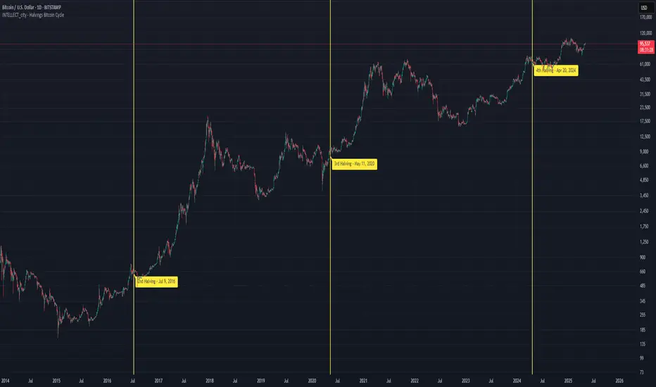
Intellect_city - Halvings Bitcoin CycleWhat is halving?
The halving timer shows when the next Bitcoin halving will occur, as well as the dates of past halvings. This event occurs every 210,000 blocks, which is approximately every 4 years. Halving reduces the emission reward by half. The original Bitcoin reward was 50 BTC per block found.
Why is halving necessary?
Halving allows you to maintain an algorithmically specified emission level. Anyone can verify that no more than 21 million bitcoins can be issued using this algorithm. Moreover, everyone can see how much was issued earlier, at what speed the emission is happening now, and how many bitcoins remain to be mined in the future. Even a sharp increase or decrease in mining capacity will not significantly affect this process. In this case, during the next difficulty recalculation, which occurs every 2014 blocks, the mining difficulty will be recalculated so that blocks are still found approximately once every ten minutes.
How does halving work in Bitcoin blocks?
The miner who collects the block adds a so-called coinbase transaction. This transaction has no entry, only exit with the receipt of emission coins to your address. If the miner's block wins, then the entire network will consider these coins to have been obtained through legitimate means. The maximum reward size is determined by the algorithm; the miner can specify the maximum reward size for the current period or less. If he puts the reward higher than possible, the network will reject such a block and the miner will not receive anything. After each halving, miners have to halve the reward they assign to themselves, otherwise their blocks will be rejected and will not make it to the main branch of the blockchain.
The impact of halving on the price of Bitcoin
It is believed that with constant demand, a halving of supply should double the value of the asset. In practice, the market knows when the halving will occur and prepares for this event in advance. Typically, the Bitcoin rate begins to rise about six months before the halving, and during the halving itself it does not change much. On average for past periods, the upper peak of the rate can be observed more than a year after the halving. It is almost impossible to predict future periods because, in addition to the reduction in emissions, many other factors influence the exchange rate. For example, major hacks or bankruptcies of crypto companies, the situation on the stock market, manipulation of “whales,” or changes in legislative regulation.
---------------------------------------------
Table - Past and future Bitcoin halvings:
---------------------------------------------
Date: Number of blocks: Award:
0 - 03-01-2009 - 0 block - 50 BTC
1 - 28-11-2012 - 210000 block - 25 BTC
2 - 09-07-2016 - 420000 block - 12.5 BTC
3 - 11-05-2020 - 630000 block - 6.25 BTC
4 - 20-04-2024 - 840000 block - 3.125 BTC
5 - 24-03-2028 - 1050000 block - 1.5625 BTC
6 - 26-02-2032 - 1260000 block - 0.78125 BTC
7 - 30-01-2036 - 1470000 block - 0.390625 BTC
8 - 03-01-2040 - 1680000 block - 0.1953125 BTC
9 - 07-12-2043 - 1890000 block - 0.09765625 BTC
10 - 10-11-2047 - 2100000 block - 0.04882813 BTC
11 - 14-10-2051 - 2310000 block - 0.02441406 BTC
12 - 17-09-2055 - 2520000 block - 0.01220703 BTC
13 - 21-08-2059 - 2730000 block - 0.00610352 BTC
14 - 25-07-2063 - 2940000 block - 0.00305176 BTC
15 - 28-06-2067 - 3150000 block - 0.00152588 BTC
16 - 01-06-2071 - 3360000 block - 0.00076294 BTC
17 - 05-05-2075 - 3570000 block - 0.00038147 BTC
18 - 08-04-2079 - 3780000 block - 0.00019073 BTC
19 - 12-03-2083 - 3990000 block - 0.00009537 BTC
20 - 13-02-2087 - 4200000 block - 0.00004768 BTC
21 - 17-01-2091 - 4410000 block - 0.00002384 BTC
22 - 21-12-2094 - 4620000 block - 0.00001192 BTC
23 - 24-11-2098 - 4830000 block - 0.00000596 BTC
24 - 29-10-2102 - 5040000 block - 0.00000298 BTC
25 - 02-10-2106 - 5250000 block - 0.00000149 BTC
26 - 05-09-2110 - 5460000 block - 0.00000075 BTC
27 - 09-08-2114 - 5670000 block - 0.00000037 BTC
28 - 13-07-2118 - 5880000 block - 0.00000019 BTC
29 - 16-06-2122 - 6090000 block - 0.00000009 BTC
30 - 20-05-2126 - 6300000 block - 0.00000005 BTC
31 - 23-04-2130 - 6510000 block - 0.00000002 BTC
32 - 27-03-2134 - 6720000 block - 0.00000001 BTC
Open Interest Inflows & Outflows [LuxAlgo]The Open Interest Inflows & Outflows indicator focuses on highlighting alterations in the overall count of active contracts associated with a specific financial instrument.
The indicator also includes an oscillator highlighting the price sentiment to use in conjunction with the open interest flow sentiment and also includes a rolling correlation of the open interest flow sentiment with a user-selected source.
🔶 USAGE
Open Interest (OI) indicates the total number of active contracts, encompassing both long and short positions, for a specific financial instrument at any given moment. This key indicator helps traders and analysts assess market activity and sentiment.
An increase in open interest generally indicates new money flowing into the market, suggesting increased activity and the potential for a trending market. Conversely, a decrease in open interest indicates that traders are closing their positions, suggesting less interest in that particular contract.
Open Interest Flow Sentiment assesses the correlation between the initiation of new positions (inflows) and the closure of existing positions (outflows) for a particular instrument. Positive values suggest a prevalence of inflows, while negative values signify a prevalence of outflows.
The magnitude of the deviation from zero reflects the extent of dominance, either in inflows or outflows.
Price Sentiment estimates the relationship between the strength of bulls (buyers) and bears (sellers) on an instrument. Positive values indicate higher bull power and negative values indicate higher bear power.
The correlation feature is a key component of the indicator and helps analyze the relationship between trading volume and Open Interest changes. If volume increases along with rising Open Interest, it supports the validity of the price trend.
A divergence between price movement, volume, and Open Interest may signal potential reversals.
🔶 DETAILS
This indicator, based on Dr. Alexander Elder's acclaimed Elder-Ray concept, aids traders in evaluating the strength of both bulls and bears by delving beneath the surface of the markets. It uncovers data not immediately apparent from a superficial glance at prices. The indicator comprises two components: Bull Power and Bear Power.
Considering that the high price of any candle signifies the maximum power of buyers and the low price represents the maximum power of sellers, Elder employs the 13-period Exponential Moving Average (EMA) to depict the average consensus of price value. Bull Power assesses whether buyers can drive prices above the average consensus of value, while Bear Power assesses whether sellers can push prices below this average.
Here are the formulas for Bull Power and Bear Power:
bull_power = high - ema(close, 13)
bear_power = low - ema(close, 13)
This concept is utilized to calculate Open Interest Flow Sentiment and Price Sentiment. The Open Interest Flow Sentiment estimates the relationship between new positions (inflows) and positions being closed (outflows), providing insights into market dynamics. The Price Sentiment, on the other hand, gauges the correlation between price movements and the Elder-Ray components, aiding traders in identifying potential shifts in market sentiment and momentum.
🔶 SETTINGS
🔹Open Interest Inflows & Outflows
OI Sentiment Correlation: toggles the visibility of Open Interest correlation with a variety of sources.
Money Flow Estimates: toggles the visibility of Money Flow Estimates calculated for the last bar.
🔹Style
OI Flow Sentiment: toggles the visibility of Open Interest Flow Sentiment, along with color customization options.
Price Sentiment: toggles the visibility of Price Sentiment, along with color customization options.
Correlation Colors: color customization option for the Correlation Area.
🔹Others
Smoothing: smoothing length applicable for Open Interest Flow Sentiment and Price Sentiment.
🔶 RELATED SCRIPTS
Open-Interest-Chart
Liquidation-Estimates
Thanks to our community for recommending this script. For more conceptual scripts and related content, we welcome you to explore by visiting >>> LuxAlgo-Scripts .

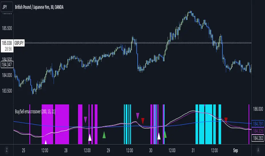
Buy/Sell EMA CrossoverThe indicator identifies potential trading opportunities within the market. It is entirely based on the combination of exponential moving averages by drawing triangles on the chart that identify buy or sell signals combined with vertical bars that create areas of interest.
Specifically, when a buy signal occurs, the indicator draws a vertical bar with an azure background, indicating a possible buy area. Similarly, a sell signal is represented by a vertical bar with a fuchsia background, indicating a possible sell area.
These areas represent the main point of the indicator which uses exponential moving averages which, based on the direction of prices, identify the trend and color the background of the graph in order to visually highlight the predominant trend.
The green triangles above the bars of the chart suggest possible upside opportunities (good bullish entry points) when the 21 ema crosses the 200 ema.
While on the contrary the red triangles, 21 ema lower than the 200 ema, can indicate possible bearish trends (good bearish entry points).
While the white and purple triangles reveal moments of potential indecision or market change.
We can think of them as situations of uncertain trend in which it is possible to place a long or short order near some conditions that we are going to see.
The white triangles below, which are created when the 13 ema is higher than the 21 ema, indicate a possible bullish zone while the purple triangles above (13 ema lower than the 21) could suggest a bearish reflex
Colored lines represent moving averages blue = 200, 21= fuchsia and 13 = white. If the price is above the 200 period line then it could be a bullish opportunity, otherwise it could be a bearish one.
An interesting strategy to adopt is to evaluate, for example, the inputs near the vertical bars (azure - long) (fuchsia - short) when a white or purple triangle appears.
The more prominent green triangle indicates that the trend is going in a long direction.
On the contrary, the red (short) triangles are the opposite of the green ones and have the same importance as input logic.
The white triangle instead present more often inside the indicator identifies interesting buying areas of short duration, it is important to consider that the closer the triangles are to the vertical blue bars the stronger the entry signal.
Finally, the purple triangles are the short-term bearish trends whose entry near the fuchsia vertical bars defines a short.
Fib TSIFib TSI = Fibonacci True Strength Index
The Fib TSI indicator uses Fibonacci numbers input for the True Strength Index moving averages. Then it is converted into a stochastic 0-100 scale.
The Fibonacci sequence is the series of numbers where each number is the sum of the two preceding numbers. 1, 2, 3, 5, 8, 13, 21, 34, 55, 89, 144, 233, 377, 610...
TSI uses moving averages of the underlying momentum of a financial instrument.
Stochastic is calculated by a formula of high and low over a length of time on a scale of 0-100.
How to use Fib TSI:
100 = overbought
0 = oversold
Rising = bullish
Falling = bearish
crossover 50 = bullish
crossunder 50 = bearish
The default input settings are:
2 = Stoch D smoothing
3 = TSI signal
TSI uses 2 moving averages compared with each other.
5 = TSI fastest
TSI uses 2 moving averages compared with each other.
Default value is 3/5.
color = white
8 = TSI fast
TSI uses 2 moving averages compared with each other.
Default value is 5/8.
color = blue
13 = TSI mid
TSI uses 2 moving averages compared with each other.
Default value is 8/13.
color = orange
21 = TSI slow
TSI uses 2 moving averages compared with each other.
Default value is 13/21.
color = purple
34 = TSI slowest
TSI uses 2 moving averages compared with each other.
Default value is 21/34.
color = yellow
55 = Stoch K length
All total / 5 = All TSI
color rising above 50 = bright green
color falling above 50 = mint green
color falling below 50 = bright red
color rising below 50 = pink
Up bullish reversal = green arrow up
bullish trend = green dots
Down bearish reversal = red arrow down
bearish trend = red dots
Horizontal lines:
100
75
50
25
0
2 different visual options example snapshot:

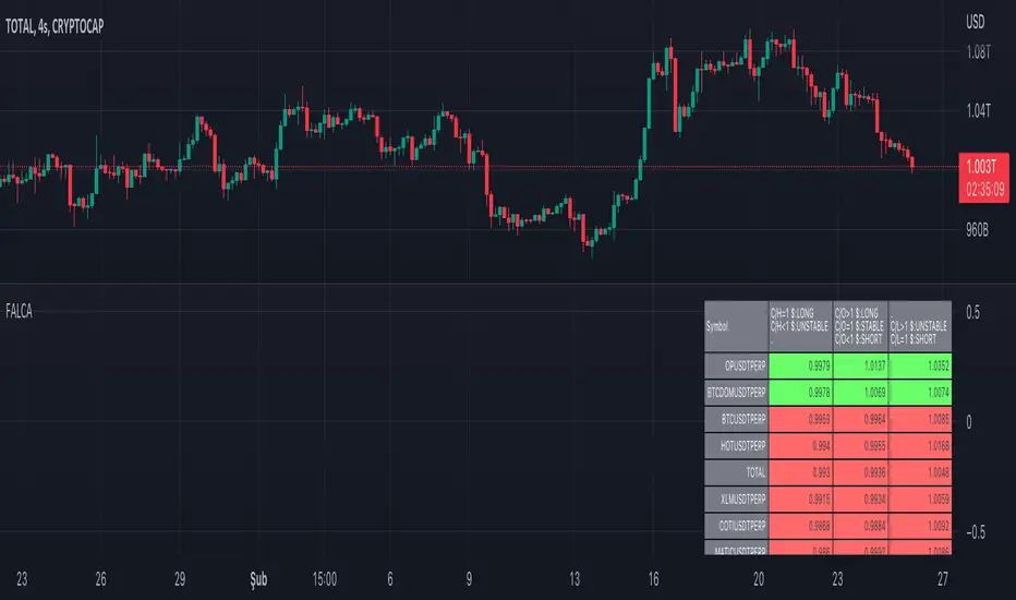
Futures All List Candle Analysis - FALCAIn this command; There is an alphabetical list of USDS-M coins with the USDT PERP extension on the Binance Futures side.
There are 13 lists in total. Each list contains 39 data. Due to data limitation, 13 lists are formed. There are 13 coins in the first 11 of the lists. The 12th list contains 3 coins. The last list (FAVORITE LIST) is CRYPTOCAP:TOTAL, BINANCE:BTCUSDTPERP, BINANCE:BTCDOMUSDTPERP as standard. You must add 10 coins to the final list.
The lists show data for the time period you selected.
Explanation of the (C/H) header: Close /High takes a maximum value of 1. As long as this value is 1, a price increase is observed.
Explanation of the (C/O) header:
Close /Open can be greater than ,1. In this case, a price increase is observed.
Close /Open can be less than 1. In this case, a price decrease is observed.
The value Close /Open can be equal to 1. In this case, price stability is observed.
Explanation of the (C/L) header: Close /Low takes a minimum value of 1. As long as this value is 1, a price decrease is observed.
Coins with a price decrease are shown in red.
Coins with a price increase will turn green.
***NOTE: For this command to work, you must first add 10 favorite coins to the "FAVORITE LIST".
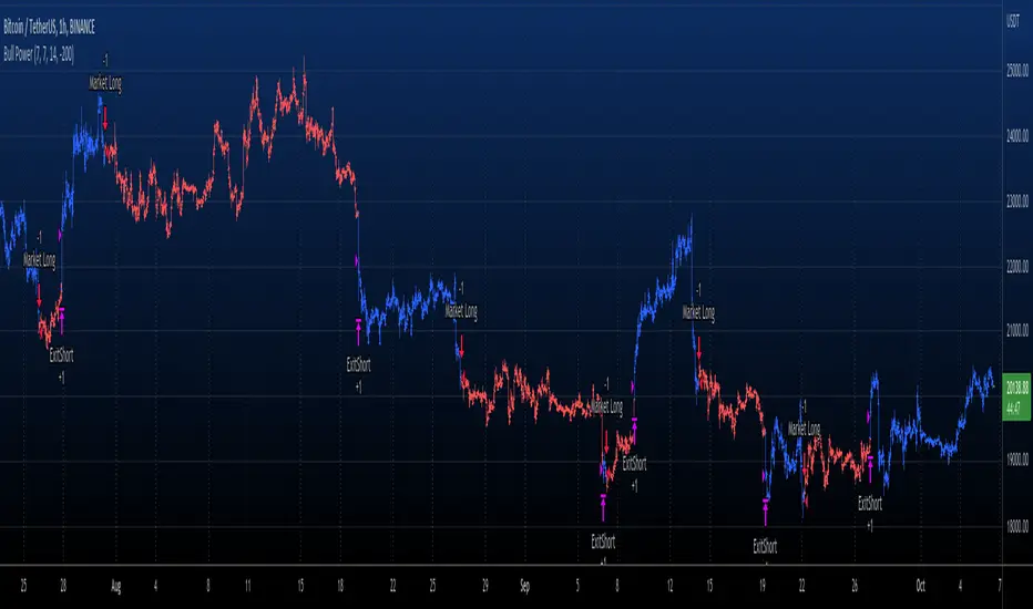
Elder Ray (Bull Power) TP and SL Developed by Dr Alexander Elder, the Elder-ray indicator measures buying
and selling pressure in the market. The Elder-ray is often used as part
of the Triple Screen trading system but may also be used on its own.
Dr Elder uses a 13-day exponential moving average (EMA) to indicate the
market consensus of value. Bull Power measures the ability of buyers to
drive prices above the consensus of value. Bear Power reflects the ability
of sellers to drive prices below the average consensus of value.
Bull Power is calculated by subtracting the 13-day EMA from the day's High.
Bear power subtracts the 13-day EMA from the day's Low.
WARNING:
- For purpose educate only
- This script to change bars colors.
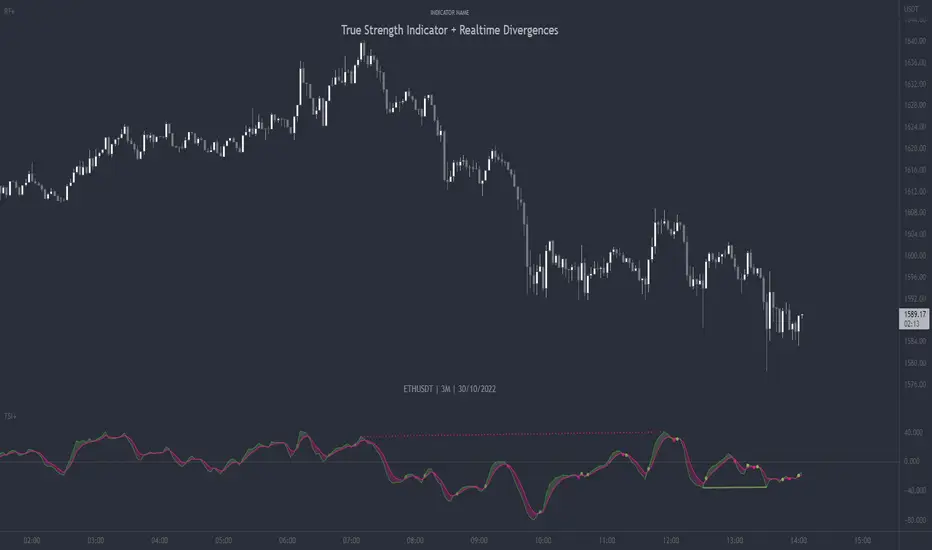
True Strength Indicator + Realtime DivergencesTrue Strength Indicator (TSI) + Realtime Divergences + Alerts + Lookback periods.
This version of the True Strength Indicator adds the following 5 additional features to the stock TSI by Tradingview:
- Optional divergence lines drawn directly onto the oscillator in realtime.
- Configurable alerts to notify you when divergences occur, as well as when the TSI and lagline bands crossover one another, when the oscillator begins heading up, or heading down.
- Configurable lookback periods to fine tune the divergences drawn in order to suit different trading styles and timeframes.
- Background colouring option to indicate when the two TSI bands, the TSI line and the TSI lagline, have crossed one another, either moving upwards or downwards, or optionally when the two TSI bands have crossed upwards and an external oscillator, which can be linked via the settings, has crossed above its centerline, and the TSI bands have crossed downwards and the external oscillator has crossed below its centerline.
- Alternate timeframe feature allows you to configure the oscillator to use data from a different timeframe than the chart it is loaded on.
This indicator adds additional features onto the stock TSI by Tradingview, whose core calculations remain unchanged, although this version has different settings as default to suit a shorter time period (it uses 6, 13, 4 by default, whereas the stock TSI typically ships with higher values, e.g. 25, 13, 13). Namely the configurable option to automatically, quickly and clearly draw divergence lines onto the oscillator for you as they occur in realtime. It also has the addition of unique alerts, so you can be notified when divergences occur without spending all day watching the charts. Furthermore, this version of the TSI comes with configurable lookback periods, which can be configured in order to adjust the sensitivity of the divergences, in order to suit shorter or higher timeframe trading approaches.
The True Strength Indicator
Tradingview describes the True Strength Indicator as follows:
“The True Strength Index (TSI) is a momentum oscillator that ranges between limits of -100 and +100 and has a base value of 0. Momentum is positive when the oscillator is positive (pointing to a bullish market bias) and vice versa. It was developed by William Blau and consists of 2 lines: the index line and an exponential moving average of the TSI, called the signal line. Traders may look for any of the following 5 types of conditions: overbought, oversold, centerline crossover, divergence and signal line crossover. The indicator is often used in combination with other signals..”
What are divergences?
Divergence is when the price of an asset is moving in the opposite direction of a technical indicator, such as an oscillator, or is moving contrary to other data. Divergence warns that the current price trend may be weakening, and in some cases may lead to the price changing direction.
There are 4 main types of divergence, which are split into 2 categories;
regular divergences and hidden divergences. Regular divergences indicate possible trend reversals, and hidden divergences indicate possible trend continuation.
Regular bullish divergence: An indication of a potential trend reversal, from the current downtrend, to an uptrend.
Regular bearish divergence: An indication of a potential trend reversal, from the current uptrend, to a downtrend.
Hidden bullish divergence: An indication of a potential uptrend continuation.
Hidden bearish divergence: An indication of a potential downtrend continuation.
Setting alerts.
With this indicator you can set alerts to notify you when any/all of the above types of divergences occur, on any chart timeframe you choose.
Configurable lookback values.
You can adjust the default lookback values to suit your prefered trading style and timeframe. If you like to trade a shorter time frame, lowering the default lookback values will make the divergences drawn more sensitive to short term price action.
How do traders use divergences in their trading?
A divergence is considered a leading indicator in technical analysis , meaning it has the ability to indicate a potential price move in the short term future.
Hidden bullish and hidden bearish divergences, which indicate a potential continuation of the current trend are sometimes considered a good place for traders to begin, since trend continuation occurs more frequently than reversals, or trend changes.
When trading regular bullish divergences and regular bearish divergences, which are indications of a trend reversal, the probability of it doing so may increase when these occur at a strong support or resistance level . A common mistake new traders make is to get into a regular divergence trade too early, assuming it will immediately reverse, but these can continue to form for some time before the trend eventually changes, by using forms of support or resistance as an added confluence, such as when price reaches a moving average, the success rate when trading these patterns may increase.
Typically, traders will manually draw lines across the swing highs and swing lows of both the price chart and the oscillator to see whether they appear to present a divergence, this indicator will draw them for you, quickly and clearly, and can notify you when they occur.
Disclaimer: This script includes code from the stock TSI by Tradingview as well as the Divergence for Many Indicators v4 by LonesomeTheBlue
Variety N-Tuple Moving Averages w/ Variety Stepping [Loxx]Variety N-Tuple Moving Averages w/ Variety Stepping is a moving average indicator that allows you to create 1- 30 tuple moving average types; i.e., Double-MA, Triple-MA, Quadruple-MA, Quintuple-MA, ... N-tuple-MA. This version contains 2 different moving average types. For example, using "50" as the depth will give you Quinquagintuple Moving Average. If you'd like to find the name of the moving average type you create with the depth input with this indicator, you can find a list of tuples here: Tuples extrapolated
Due to the coding required to adapt a moving average to fit into this indicator, additional moving average types will be added as they are created to fit into this unique use case. Since this is a work in process, there will be many future updates of this indicator. For now, you can choose from either EMA or RMA.
This indicator is also considered one of the top 10 forex indicators. See details here: forex-station.com
Additionally, this indicator is a computationally faster, more streamlined version of the following indicators with the addition of 6 stepping functions and 6 different bands/channels types.
STD-Stepped, Variety N-Tuple Moving Averages
STD-Stepped, Variety N-Tuple Moving Averages is the standard deviation stepped/filtered indicator of the following indicator
Last but not least, a big shoutout to @lejmer for his help in formulating a looping solution for this streamlined version. this indicator is speedy even at 50 orders deep. You can find his scripts here: www.tradingview.com
How this works
Step 1: Run factorial calculation on the depth value,
Step 2: Calculate weights of nested moving averages
factorial(depth) / (factorial(depth - k) * factorial(k); where depth is the depth and k is the weight position
Examples of coefficient outputs:
6 Depth: 6 15 20 15 6
7 Depth: 7 21 35 35 21 7
8 Depth: 8 28 56 70 56 28 8
9 Depth: 9 36 34 84 126 126 84 36 9
10 Depth: 10 45 120 210 252 210 120 45 10
11 Depth: 11 55 165 330 462 462 330 165 55 11
12 Depth: 12 66 220 495 792 924 792 495 220 66 12
13 Depth: 13 78 286 715 1287 1716 1716 1287 715 286 78 13
Step 3: Apply coefficient to each moving average
For QEMA, which is 5 depth EMA , the calculation is as follows
ema1 = ta. ema ( src , length)
ema2 = ta. ema (ema1, length)
ema3 = ta. ema (ema2, length)
ema4 = ta. ema (ema3, length)
ema5 = ta. ema (ema4, length)
In this new streamlined version, these MA calculations are packed into an array inside loop so Pine doesn't have to keep all possible series information in memory. This is handled with the following code:
temp = array.get(workarr, k + 1) + alpha * (array.get(workarr, k) - array.get(workarr, k + 1))
array.set(workarr, k + 1, temp)
After we pack the array, we apply the coefficients to derive the NTMA:
qema = 5 * ema1 - 10 * ema2 + 10 * ema3 - 5 * ema4 + ema5
Stepping calculations
First off, you can filter by both price and/or MA output. Both price and MA output can be filtered/stepped in their own way. You'll see two selectors in the input settings. Default is ATR ATR. Here's how stepping works in simple terms: if the price/MA output doesn't move by X deviations, then revert to the price/MA output one bar back.
ATR
The average true range (ATR) is a technical analysis indicator, introduced by market technician J. Welles Wilder Jr. in his book New Concepts in Technical Trading Systems, that measures market volatility by decomposing the entire range of an asset price for that period.
Standard Deviation
Standard deviation is a statistic that measures the dispersion of a dataset relative to its mean and is calculated as the square root of the variance. The standard deviation is calculated as the square root of variance by determining each data point's deviation relative to the mean. If the data points are further from the mean, there is a higher deviation within the data set; thus, the more spread out the data, the higher the standard deviation.
Adaptive Deviation
By definition, the Standard Deviation (STD, also represented by the Greek letter sigma σ or the Latin letter s) is a measure that is used to quantify the amount of variation or dispersion of a set of data values. In technical analysis we usually use it to measure the level of current volatility .
Standard Deviation is based on Simple Moving Average calculation for mean value. This version of standard deviation uses the properties of EMA to calculate what can be called a new type of deviation, and since it is based on EMA , we can call it EMA deviation. And added to that, Perry Kaufman's efficiency ratio is used to make it adaptive (since all EMA type calculations are nearly perfect for adapting).
The difference when compared to standard is significant--not just because of EMA usage, but the efficiency ratio makes it a "bit more logical" in very volatile market conditions.
See how this compares to Standard Devaition here:
Adaptive Deviation
Median Absolute Deviation
The median absolute deviation is a measure of statistical dispersion. Moreover, the MAD is a robust statistic, being more resilient to outliers in a data set than the standard deviation. In the standard deviation, the distances from the mean are squared, so large deviations are weighted more heavily, and thus outliers can heavily influence it. In the MAD, the deviations of a small number of outliers are irrelevant.
Because the MAD is a more robust estimator of scale than the sample variance or standard deviation, it works better with distributions without a mean or variance, such as the Cauchy distribution.
For this indicator, I used a manual recreation of the quantile function in Pine Script. This is so users have a full inside view into how this is calculated.
Efficiency-Ratio Adaptive ATR
Average True Range (ATR) is widely used indicator in many occasions for technical analysis . It is calculated as the RMA of true range. This version adds a "twist": it uses Perry Kaufman's Efficiency Ratio to calculate adaptive true range
See how this compares to ATR here:
ER-Adaptive ATR
Mean Absolute Deviation
The mean absolute deviation (MAD) is a measure of variability that indicates the average distance between observations and their mean. MAD uses the original units of the data, which simplifies interpretation. Larger values signify that the data points spread out further from the average. Conversely, lower values correspond to data points bunching closer to it. The mean absolute deviation is also known as the mean deviation and average absolute deviation.
This definition of the mean absolute deviation sounds similar to the standard deviation (SD). While both measure variability, they have different calculations. In recent years, some proponents of MAD have suggested that it replace the SD as the primary measure because it is a simpler concept that better fits real life.
For Pine Coders, this is equivalent of using ta.dev()
Bands/Channels
See the information above for how bands/channels are calculated. After the one of the above deviations is calculated, the channels are calculated as output +/- deviation * multiplier
Signals
Green is uptrend, red is downtrend, yellow "L" signal is Long, fuchsia "S" signal is short.
Included:
Alerts
Loxx's Expanded Source Types
Bar coloring
Signals
6 bands/channels types
6 stepping types
Related indicators
3-Pole Super Smoother w/ EMA-Deviation-Corrected Stepping
STD-Stepped Fast Cosine Transform Moving Average
ATR-Stepped PDF MA

STD-Stepped, Variety N-Tuple Moving Averages [Loxx]STD-Stepped, Variety N-Tuple Moving Averages is the standard deviation stepped/filtered indicator of the following indicator
Variety N-Tuple Moving Averages is a moving average indicator that allows you to create 1- 30 tuple moving average types; i.e., Double-MA, Triple-MA, Quadruple-MA, Quintuple-MA, ... N-tuple-MA. This version contains 5 different moving average types including T3. A list of tuples can be found here if you'd like to name the order of the moving average by depth: Tuples extrapolated
STD-Stepped, You'll notice that this is a lot of code and could normally be packed into a single loop in order to extract the N-tuple MA, however due to Pine Script limitations and processing paradigm this is not possible ... yet.
If you choose the EMA option and select a depth of 2, this is the classic DEMA ; EMA with a depth of 3 is the classic TEMA , and so on and so forth this is to help you understand how this indicator works. This version of NTMA is restricted to a maximum depth of 30 or less. Normally this indicator would include 50 depths but I've cut this down to 30 to reduce indicator load time. In the future, I'll create an updated NTMA that allows for more depth levels.
This is considered one of the top ten indicators in forex. You can read more about it here: forex-station.com
How this works
Step 1: Run factorial calculation on the depth value,
Step 2: Calculate weights of nested moving averages
factorial(nemadepth) / (factorial(nemadepth - k) * factorial(k); where nemadepth is the depth and k is the weight position
Examples of coefficient outputs:
6 Depth: 6 15 20 15 6
7 Depth: 7 21 35 35 21 7
8 Depth: 8 28 56 70 56 28 8
9 Depth: 9 36 34 84 126 126 84 36 9
10 Depth: 10 45 120 210 252 210 120 45 10
11 Depth: 11 55 165 330 462 462 330 165 55 11
12 Depth: 12 66 220 495 792 924 792 495 220 66 12
13 Depth: 13 78 286 715 1287 1716 1716 1287 715 286 78 13
Step 3: Apply coefficient to each moving average
For QEMA, which is 5 depth EMA , the caculation is as follows
ema1 = ta. ema ( src , length)
ema2 = ta. ema (ema1, length)
ema3 = ta. ema (ema2, length)
ema4 = ta. ema (ema3, length)
ema5 = ta. ema (ema4, length)
qema = 5 * ema1 - 10 * ema2 + 10 * ema3 - 5 * ema4 + ema5
Included:
Alerts
Loxx's Expanded Source Types
Bar coloring
Signals
Standard deviation stepping

Variety N-Tuple Moving Averages [Loxx]Variety N-Tuple Moving Averages is a moving average indicator that allows you to create 1- 30 tuple moving average types; i.e., Double-MA, Triple-MA, Quadruple-MA, Quintuple-MA, ... N-tuple-MA. This version contains 5 different moving average types including T3. A list of tuples can be found here if you'd like to name the order of the moving average by depth: Tuples extrapolated
You'll notice that this is a lot of code and could normally be packed into a single loop in order to extract the N-tuple MA, however due to Pine Script limitations and processing paradigm this is not possible ... yet.
If you choose the EMA option and select a depth of 2, this is the classic DEMA; EMA with a depth of 3 is the classic TEMA, and so on and so forth this is to help you understand how this indicator works. This version of NTMA is restricted to a maximum depth of 30 or less. Normally this indicator would include 50 depths but I've cut this down to 30 to reduce indicator load time. In the future, I'll create an updated NTMA that allows for more depth levels.
This is considered one of the top ten indicators in forex. You can read more about it here: forex-station.com
How this works
Step 1: Run factorial calculation on the depth value,
Step 2: Calculate weights of nested moving averages
factorial(nemadepth) / (factorial(nemadepth - k) * factorial(k); where nemadepth is the depth and k is the weight position
Examples of coefficient outputs:
6 Depth: 6 15 20 15 6
7 Depth: 7 21 35 35 21 7
8 Depth: 8 28 56 70 56 28 8
9 Depth: 9 36 34 84 126 126 84 36 9
10 Depth: 10 45 120 210 252 210 120 45 10
11 Depth: 11 55 165 330 462 462 330 165 55 11
12 Depth: 12 66 220 495 792 924 792 495 220 66 12
13 Depth: 13 78 286 715 1287 1716 1716 1287 715 286 78 13
Step 3: Apply coefficient to each moving average
For QEMA, which is 5 depth EMA, the caculation is as follows
ema1 = ta.ema(src, length)
ema2 = ta.ema(ema1, length)
ema3 = ta.ema(ema2, length)
ema4 = ta.ema(ema3, length)
ema5 = ta.ema(ema4, length)
qema = 5 * ema1 - 10 * ema2 + 10 * ema3 - 5 * ema4 + ema5
Included:
Alerts
Loxx's Expanded Source Types
Bar coloring
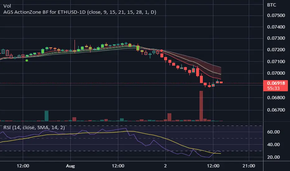
CDC ActionZone BF for ETHUSD-1D © PRoSkYNeT-EE
Based on improvements from "Kitti-Playbook Action Zone V.4.2.0.3 for Stock Market"
Based on improvements from "CDC Action Zone V3 2020 by piriya33"
Based on Triple MACD crossover between 9/15, 21/28, 15/28 for filter error signal (noise) from CDC ActionZone V3
MACDs generated from the execution of millions of times in the "Brute Force Algorithm" to backtest data from the past 5 years. ( 2017-08-21 to 2022-08-01 )
Released 2022-08-01
***** The indicator is used in the ETHUSD 1 Day period ONLY *****
Recommended Stop Loss : -4 % (execute stop Loss after candlestick has been closed)
Backtest Result ( Start $100 )
Winrate 63 % (Win:12, Loss:7, Total:19)
Live Days 1,806 days
B : Buy
S : Sell
SL : Stop Loss
2022-07-19 07 - 1,542 : B 6.971 ETH
2022-04-13 07 - 3,118 : S 8.98 % $10,750 12,7,19 63 %
2022-03-20 07 - 2,861 : B 3.448 ETH
2021-12-03 07 - 4,216 : SL -8.94 % $9,864 11,7,18 61 %
2021-11-30 07 - 4,630 : B 2.340 ETH
2021-11-18 07 - 3,997 : S 13.71 % $10,832 11,6,17 65 %
2021-10-05 07 - 3,515 : B 2.710 ETH
2021-09-20 07 - 2,977 : S 29.38 % $9,526 10,6,16 63 %
2021-07-28 07 - 2,301 : B 3.200 ETH
2021-05-20 07 - 2,769 : S 50.49 % $7,363 9,6,15 60 %
2021-03-30 07 - 1,840 : B 2.659 ETH
2021-03-22 07 - 1,681 : SL -8.29 % $4,893 8,6,14 57 %
2021-03-08 07 - 1,833 : B 2.911 ETH
2021-02-26 07 - 1,445 : S 279.27 % $5,335 8,5,13 62 %
2020-10-13 07 - 381 : B 3.692 ETH
2020-09-05 07 - 335 : S 38.43 % $1,407 7,5,12 58 %
2020-07-06 07 - 242 : B 4.199 ETH
2020-06-27 07 - 221 : S 28.49 % $1,016 6,5,11 55 %
2020-04-16 07 - 172 : B 4.598 ETH
2020-02-29 07 - 217 : S 47.62 % $791 5,5,10 50 %
2020-01-12 07 - 147 : B 3.644 ETH
2019-11-18 07 - 178 : S -2.73 % $536 4,5,9 44 %
2019-11-01 07 - 183 : B 3.010 ETH
2019-09-23 07 - 201 : SL -4.29 % $551 4,4,8 50 %
2019-09-18 07 - 210 : B 2.740 ETH
2019-07-12 07 - 275 : S 63.69 % $575 4,3,7 57 %
2019-05-03 07 - 168 : B 2.093 ETH
2019-04-28 07 - 158 : S 29.51 % $352 3,3,6 50 %
2019-02-15 07 - 122 : B 2.225 ETH
2019-01-10 07 - 125 : SL -6.02 % $271 2,3,5 40 %
2018-12-29 07 - 133 : B 2.172 ETH
2018-05-22 07 - 641 : S 5.95 % $289 2,2,4 50 %
2018-04-21 07 - 605 : B 0.451 ETH
2018-02-02 07 - 922 : S 197.42 % $273 1,2,3 33 %
2017-11-11 07 - 310 : B 0.296 ETH
2017-10-09 07 - 297 : SL -4.50 % $92 0,2,2 0 %
2017-10-07 07 - 311 : B 0.309 ETH
2017-08-22 07 - 310 : SL -4.02 % $96 0,1,1 0 %
2017-08-21 07 - 323 : B 0.310 ETH
StapleIndicatorsLibrary "StapleIndicators"
This Library provides some common indicators commonly referenced from other studies in Pine Script
squeeze(bbSrc, bbPeriod, bbDev, kcSrc, kcPeriod, kcATR, signalPeriod) Volatility Squeeze
Parameters:
bbSrc : (Optional) Bollinger Bands Source. By default close
bbPeriod : (Optional) Bollinger Bands Period. By default 20
bbDev : (Optional) Bollinger Bands Standard Deviation. By default 2.0
kcSrc : (Optional) Keltner Channel Source. By default close
kcPeriod : (Optional) Keltner Channel Period. By default 20
kcATR : (Optional) Keltner Channel ATR Multiplier. By default 1.5
signalPeriod : (Optional) Keltner Channel ATR Multiplier. By default 1.5
Returns:
adx(diPeriod, adxPeriod, signalPeriod, adxTier1, adxTier2, adxTier3) ADX: Average Directional Index
Parameters:
diPeriod : (Optional) Directional Indicator Period. By default 14
adxPeriod : (Optional) ADX Smoothing. By default 14
signalPeriod : (Optional) Signal Period. By default 13
adxTier1 : (Optional) ADX Tier #1 Level. By default 20
adxTier2 : (Optional) ADX Tier #2 Level. By default 15
adxTier3 : (Optional) ADX Tier #3 Level. By default 10
Returns:
smaPreset(srcMa) Delivers a set of frequently used Simple Moving Averages
Parameters:
srcMa : (Optional) MA Source. By default 'close'
Returns:
emaPreset(srcMa) Delivers a set of frequently used Exponential Moving Averages
Parameters:
srcMa : (Optional) MA Source. By default 'close'
Returns:
maSelect(ma, srcMa) Filters and outputs the selected MA
Parameters:
ma : (Optional) MA text. By default 'Ema-21'
srcMa : (Optional) MA Source. By default 'close'
Returns: maSelected
periodAdapt(modeAdaptative, src, maxLen, minLen) Adaptative Period
Parameters:
modeAdaptative : (Optional) Adaptative Mode. By default 'Average'
src : (Optional) Source. By default 'close'
maxLen : (Optional) Max Period. By default '60'
minLen : (Optional) Min Period. By default '4'
Returns: periodAdaptative
azlema(modeAdaptative, srcMa) Azlema: Adaptative Zero-Lag Ema
Parameters:
modeAdaptative : (Optional) Adaptative Mode. By default 'Average'
srcMa : (Optional) MA Source. By default 'close'
Returns: azlema
ssma(lsmaVar, srcMa, periodMa) SSMA: Smooth Simple MA
Parameters:
lsmaVar : Linear Regression Curve.
srcMa : (Optional) MA Source. By default 'close'
periodMa : (Optional) MA Period. By default '13'
Returns: ssma
jvf(srcMa, periodMa) Jurik Volatility Factor
Parameters:
srcMa : (Optional) MA Source. By default 'close'
periodMa : (Optional) MA Period. By default '7'
Returns:
jBands(srcMa, periodMa) Jurik Bands
Parameters:
srcMa : (Optional) MA Source. By default 'close'
periodMa : (Optional) MA Period. By default '7'
Returns:
jma(srcMa, periodMa, phase) Jurik MA (JMA)
Parameters:
srcMa : (Optional) MA Source. By default 'close'
periodMa : (Optional) MA Period. By default '7'
phase : (Optional) Phase. By default '50'
Returns: jma
maCustom(ma, srcMa, periodMa, lrOffset, almaOffset, almaSigma, jmaPhase, azlemaMode) Creates a custom Moving Average
Parameters:
ma : (Optional) MA text. By default 'Ema'
srcMa : (Optional) MA Source. By default 'close'
periodMa : (Optional) MA Period. By default '13'
lrOffset : (Optional) Linear Regression Offset. By default '0'
almaOffset : (Optional) Alma Offset. By default '0.85'
almaSigma : (Optional) Alma Sigma. By default '6'
jmaPhase : (Optional) JMA Phase. By default '50'
azlemaMode : (Optional) Azlema Adaptative Mode. By default 'Average'
Returns: maTF

+ Magic Carpet BandsFun name for an indicator, eh? Well, it is true, I think; they look like magic carpets. They're actually pretty simple actually. They're Keltner Channels smoothed with a moving average. If you go down to the lookback period for the bands and set it to 1, you'll recognize them immediately.
Digging a bit deeper you see there are four magic carpets on the chart. The inner ones are set to a multiplier of 2, and the outer to a multiplier of 4. Each "carpet" is composed of two smoothed upper or lower Keltner Channels bounds, both with an optional offset, one of which is set to 13, and the other to 0 by default; and an optional color fill between these. There is also a color fill between the outer and inner carpets which gives them an interesting 3-dimensional aspect at times. They can look a bit like tunnels by default.
My thinking around the idea of using an offset with the bands is that if we assume these things to provide a dynamic support and resistance, and previous support and resistance maintains status as support and resistance until proven otherwise, then by putting an offset to past data we are creating a more obvious visual indication of that support or resistance in the present. The default offset is set to 13 bars back, so if price found resistance at some point around 13 bars ago, and price is currently revisiting it we assume it is still resistance, and that offset band is there to give us a strong visual aid. Obviously it's not foolproof, but nothing is.
Beyond that most interesting part of the indicator you have a nice selection of moving averages which the bands are calculated off of. By default it's set to my UMA. The bands themselves also have a selection of moving averages for how the keltner channels are smoothed. And a note: because the UMA and RDMA are averages of different length MAs, they can not be adjusted other than via the multiplier that sets the distance from the moving average.
The indicator is multi-timeframe, and the moving average can be colored based on a higher timeframe as well.
I popped in the divergence indicator here too. You can choose from RSI and OBV, and the divergences will be plotted on the chart. Working on finding a way to be able to have the bands/MA set to a higher timeframe while plotting the divergences on the chart timeframe, but don't have an answer to that yet.
Alerts for moving average crosses, band touches, and divergences.
I like this one a lot. Enjoy!
Pictures below.
s3.tradingview.com
One interesting thing about this indicator is that band twists often occur at areas of support or resistance. Simply drawing horizontal lines from previous twisted points can provide places from which you may look for strength or weakness to enter into a trade, or which you might use as targets for taking profits. The vertical lines are just showing the point on the chart when the cross occurred.
s3.tradingview.com
Above is a Jurik MA with a bunch of adjustments made to the bands, and the moving average itself. Everything is super adjustable, so you can play around and have fun with them quite a bit.
s3.tradingview.com
Just a different MA and bands.
s3.tradingview.com

Ultimate Multi-MACD - Early Warnings + Main TrendThis is a set of a bunch of moving averages. Unique, huh? Right. Awesome. Dope.
So, what's cool about this set, is its usability as not just one MACD, but a pair of MACDs specifically tuned to keep you hard. Some of you probably notice already just looking at the available MAs and lengths - there are some common pairs here. But what do you get when you combine all these common pairs that share bases? You get both short and long term plays out of it. The thing MACDs aren't supposed to do. I imagine it would be hard to make a backtestable/bottable script version of this, because the main thing is you have to use your gut a little bit in determing when to take a short term play and when to keep to the long term plays.
In this set, you get 3 TEMAs, 2 VWMAs, 2 SMAs, and 2 ALMAs. Yeah. That's almost TOO phat. I know. Whatever.
The two purple/pink lines are your 25 VWMA and 50 ALMA slow lines. These will be your main slow lines. They're usually close but move around a decent bit and if you want you could make buys and sales using the Alma crossing above the VWMA as a buy and sell crossing under.
Then you have a THIRD potential slow line on your dark green 50 TEMA. You generally use either the 13 or 21 TEMA crossing up as buy and down as sell. The signal TEMAs are bright green 13 and yellow 21.
Next you have all your Fast signal MAs! A peachy 10 VWMA, 13 green TEMA, 21 yellow TEMA, 10 teal/bright blue ALMA and last but not least, two pale SMAs at 5 and 10. The 5 could even be used as a signal against the 10 if you really want. There are countless options for buy and sell signals. Hide and show the ones that work the best on the chart you're trading on. Different ones will work different times. Why not see which ones are working BEST out of all the best ones, though?
Please leave other MA pairs that you would like added in future versions. If I do make a future version with more pairs I will very likely set default to hide some
Enjoy.
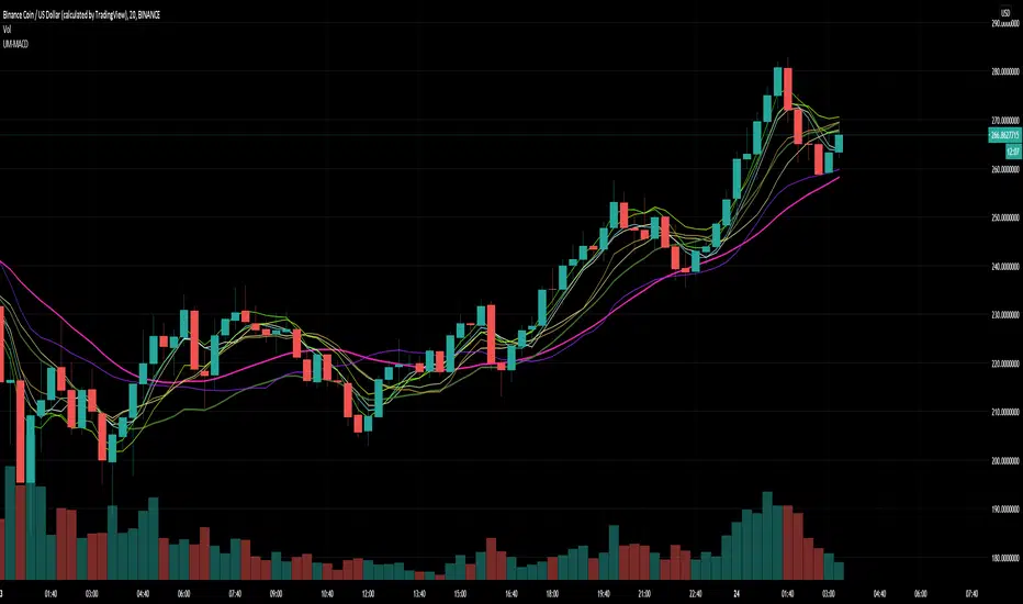
Time Divergence - TDV [SHK]A truly time based indicator to check the strength of the asset based on "Time". The main idea came to my mind about 2 years ago, When i was counting the candles in an impulse move and comparing it to number of retracement candles .
So i got a period (13 for example) and checked the price change between the 13 candles, Then the space between those two points (the price!) is divided to 13 (the time!).
The result can be analyzed by checking the Divergence, or checking the Linear Regression, or bollinger band, or trend lines and channels, or ...
You can also test different periods.
I'm price action trader and i don't use indicators, But i publish my past works for other users.
Hope you find new usage methods and share them in comments.

Aroon Oscillator StrategyThis is simple strategy based on Aroon Oscillator. I have found that using length 144 or 169 on hourly chart shows excellent results.
Tested on SPY , QQQ and AAPL. Especially when you look at AAPL results , it has 60% profitable in recent trades. ( Dont assume this will be same for other stocks or ETFs)
Aroon Oscillator setting : 169 ( 169 is square root of 13 ... you can also use fib level 144 , which is square root of 12 )
BUY
When Aroon Oscillator crosses above zero line
Add
if Long position is already opened, and current close is less than BUY price and RSI 13 crossing above 30 line
Exit
when Aroon Oscialltor crosses below zero line
Stop Loss
default stop loss has been set to 5%
Note: I have not plotted RSI to the chart. Please include RSI 13 to see how position gets added ... Also add ema 169 to see how the price is aligned with the Aroon Oscillator
Warning
For the educational purposes only

Combo Backtest 123 Reversal & Elder Ray (Bull Power) This is combo strategies for get a cumulative signal.
First strategy
This System was created from the Book "How I Tripled My Money In The
Futures Market" by Ulf Jensen, Page 183. This is reverse type of strategies.
The strategy buys at market, if close price is higher than the previous close
during 2 days and the meaning of 9-days Stochastic Slow Oscillator is lower than 50.
The strategy sells at market, if close price is lower than the previous close price
during 2 days and the meaning of 9-days Stochastic Fast Oscillator is higher than 50.
Second strategy
Developed by Dr Alexander Elder, the Elder-ray indicator measures buying
and selling pressure in the market. The Elder-ray is often used as part
of the Triple Screen trading system but may also be used on its own.
Dr Elder uses a 13-day exponential moving average (EMA) to indicate the
market consensus of value. Bull Power measures the ability of buyers to
drive prices above the consensus of value. Bear Power reflects the ability
of sellers to drive prices below the average consensus of value.
Bull Power is calculated by subtracting the 13-day EMA from the day's High.
Bear power subtracts the 13-day EMA from the day's Low.
You can use in the xPrice any series: Open, High, Low, Close, HL2, HLC3, OHLC4 and ect...
WARNING:
- For purpose educate only
- This script to change bars colors.

Combo Strategy 123 Reversal & Elder Ray (Bull Power) This is combo strategies for get a cumulative signal.
First strategy
This System was created from the Book "How I Tripled My Money In The
Futures Market" by Ulf Jensen, Page 183. This is reverse type of strategies.
The strategy buys at market, if close price is higher than the previous close
during 2 days and the meaning of 9-days Stochastic Slow Oscillator is lower than 50.
The strategy sells at market, if close price is lower than the previous close price
during 2 days and the meaning of 9-days Stochastic Fast Oscillator is higher than 50.
Second strategy
Developed by Dr Alexander Elder, the Elder-ray indicator measures buying
and selling pressure in the market. The Elder-ray is often used as part
of the Triple Screen trading system but may also be used on its own.
Dr Elder uses a 13-day exponential moving average (EMA) to indicate the
market consensus of value. Bull Power measures the ability of buyers to
drive prices above the consensus of value. Bear Power reflects the ability
of sellers to drive prices below the average consensus of value.
Bull Power is calculated by subtracting the 13-day EMA from the day's High.
Bear power subtracts the 13-day EMA from the day's Low.
You can use in the xPrice any series: Open, High, Low, Close, HL2, HLC3, OHLC4 and ect...
WARNING:
- For purpose educate only
- This script to change bars colors.

Combo Backtest 123 Reversal & Elder Ray (Bear Power) This is combo strategies for get a cumulative signal.
First strategy
This System was created from the Book "How I Tripled My Money In The
Futures Market" by Ulf Jensen, Page 183. This is reverse type of strategies.
The strategy buys at market, if close price is higher than the previous close
during 2 days and the meaning of 9-days Stochastic Slow Oscillator is lower than 50.
The strategy sells at market, if close price is lower than the previous close price
during 2 days and the meaning of 9-days Stochastic Fast Oscillator is higher than 50.
Second strategy
Developed by Dr Alexander Elder, the Elder-ray indicator measures buying
and selling pressure in the market. The Elder-ray is often used as part
of the Triple Screen trading system but may also be used on its own.
Dr Elder uses a 13-day exponential moving average (EMA) to indicate the
market consensus of value. Bull Power measures the ability of buyers to
drive prices above the consensus of value. Bear Power reflects the ability
of sellers to drive prices below the average consensus of value.
Bull Power is calculated by subtracting the 13-day EMA from the day's High.
Bear power subtracts the 13-day EMA from the day's Low.
You can use in the xPrice any series: Open, High, Low, Close, HL2, HLC3, OHLC4 and ect...
WARNING:
- For purpose educate only
- This script to change bars colors.
