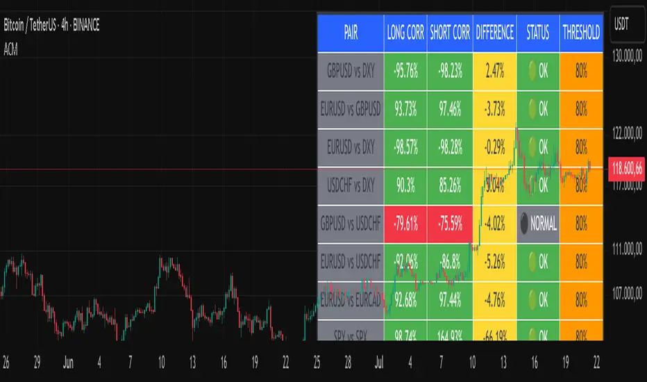
Advanced Correlation Monitor📊 Advanced Correlation Monitor - Pine Script v6
🎯 What does this indicator do?
Monitors real-time correlations between 13 different asset pairs and alerts you when historically strong correlations break, indicating potential trading opportunities or changes in market dynamics.
🚀 Key Features
✨ Multi-Market Monitoring
7 Forex Pairs (GBPUSD/DXY, EURUSD/GBPUSD, etc.)
6 Index/Stock Pairs (SPY/S&P500, DAX/NASDAQ, TSLA/NVDA, etc.)
Fully configurable - change any pair from inputs
📈 Dual Correlation Analysis
Long Period (90 bars): Identifies historically strong correlations
Short Period (6 bars): Detects recent breakdowns
Pearson Correlation using Pine Script v6 native functions
🎨 Intuitive Visualization
Real-time table with 6 information columns
Color coding: Green (correlated), Red (broken), Gray (normal)
Visual states: 🟢 OK, 🔴 BROKEN, ⚫ NORMAL
🚨 Smart Alert System
Only alerts previously correlated pairs (>80% historical)
Detects breakdowns when short correlation <80%
Consolidated alert with all affected pairs
🛠️ Flexible Configuration
Adjustable Parameters:
📅 Periods: Long (30-500), Short (2-50)
🎯 Threshold: 50%-99% (default 80%)
🎨 Table: Configurable position and size
📊 Symbols: All pairs are configurable
Default Pairs:
FOREX: INDICES/STOCKS:
- GBPUSD vs DXY • SPY vs S&P500
- EURUSD vs GBPUSD • DAX vs S&P500
- EURUSD vs DXY • DAX vs NASDAQ
- USDCHF vs DXY • TSLA vs NVDA
- GBPUSD vs USDCHF • MSFT vs NVDA
- EURUSD vs USDCHF • AAPL vs NVDA
- EURUSD vs EURCAD
💡 Practical Use Cases
🔄 Pairs Trading
Detects when strong correlations break for:
Statistical arbitrage
Mean reversion trading
Divergence opportunities
🛡️ Risk Management
Identifies when "safe" assets start moving independently:
Portfolio diversification
Smart hedging
Regime change detection
📊 Market Analysis
Understand underlying market structure:
Forex/DXY correlations
Tech sector rotation
Regional market disconnection
🎓 Results Interpretation
Reading Example:
EURUSD vs DXY: -98.57% → -98.27% | 🟢 OK
└─ Perfect negative correlation maintained (EUR rises when DXY falls)
TSLA vs NVDA: 78.12% → 0% | ⚫ NORMAL
└─ Lost tech correlation (divergence opportunity)
Trading Signals:
🟢 → 🔴: Broken correlation = Possible opportunity
Large difference: Indicates correlation tension
Multiple breaks: Market regime change
Wyszukaj w skryptach "细算江西救护车家长倒赚了四万三+-医疗花费13万(家长视频)++医保报"
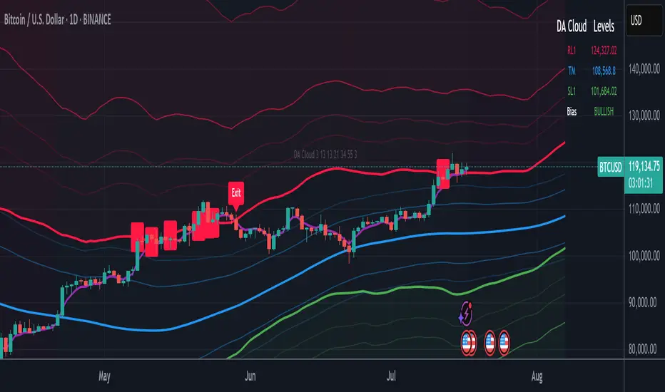
DA Cloud - DynamicDA Cloud - Dynamic | Detailed Overview
🌟 What Makes This Indicator Special
The DA Cloud - Dynamic is an advanced technical analysis tool that creates adaptive support and resistance zones that expand and contract based on market volatility. Unlike traditional static indicators, this cloud system "breathes" with the market, providing dynamic levels that adjust to changing market conditions.
📊 Core Components
1. Multi-Layered Cloud Structure
Resistance Cloud (Red): Three dynamic resistance levels (RL1, RL2, RL3) with intermediate channels (RC1, RC2)
Support Cloud (Green): Three dynamic support levels (SL1, SL2, SL3) with intermediate channels (SC1, SC2)
Trend Cloud (Blue): Five trend lines (TU2, TU1, TM, TL1, TL2) that flow through the center
Confirmation Line (Purple): A fast-reacting line that confirms trend changes
2. Forward Displacement Technology
The entire cloud system is projected 21 bars into the future (Fibonacci number), allowing traders to see potential support and resistance levels before price reaches them. This predictive element is inspired by Ichimoku Cloud theory but enhanced with modern volatility dynamics.
🔬 How It Works (Without Revealing the Secret Sauce)
Volatility-Responsive Design
The indicator continuously measures market volatility across multiple timeframes
During high volatility periods (like major breakouts), clouds expand dramatically
During consolidation, clouds contract and tighten around price
This creates a "breathing" effect that adapts to market conditions
Multi-Timeframe Analysis
Incorporates Fibonacci sequence periods (3, 13, 21, 34, 55) for calculations
Blends short-term responsiveness with long-term stability
Creates smooth, flowing lines that filter out market noise
Dynamic Level Calculation
Levels are not fixed percentages or static bands
Each level adapts based on current market structure and volatility
Channel lines (RC1, RC2, SC1, SC2) provide intermediate support/resistance
🎯 Key Features
1. Touch Point Detection
Colored dots appear when price touches key levels
Red dots = resistance touch
Green dots = support touch
Blue dots = trend median touch
2. Entry/Exit Signals
"Cloud Entry" labels when confirmation line crosses above SL1
"Cloud Exit" labels when confirmation line crosses below RL1
Background color changes based on bullish/bearish bias
3. Information Table
Real-time display of key levels (RL1, TM, SL1)
Current bias indicator (BULLISH/BEARISH)
Updates dynamically as market moves
⚙️ Customization Options
Main Controls:
Sensitivity (5-50): How responsive clouds are to price movements
Smoothing (1-50): Controls the flow and smoothness of cloud lines
Forward Displacement (0-50): How many bars to project the cloud forward
Advanced Volatility Settings:
Volatility Lookback (50-1000): Period for establishing volatility baseline
Volatility Smoothing (1-50): Reduces spikes in volatility expansion
Expansion Power (0.1-2.0): Controls how dramatically clouds expand
Range Divisor (1.0-20.0): Master control for overall cloud width
Level Spacing:
Individual multipliers for each resistance and support level
Allows fine-tuning of cloud structure to match different markets
Trend Spacing:
Separate controls for inner and outer trend bands
Customize the trend cloud density
📈 Trading Applications
1. Trend Identification
Price above TM (Trend Median) = Bullish bias
Price below TM = Bearish bias
Cloud color and width indicate trend strength
2. Support/Resistance Trading
Use RL1/SL1 as primary targets and reversal zones
RC1/RC2 and SC1/SC2 provide intermediate levels
RL3/SL3 mark extreme levels often seen at major tops/bottoms
3. Volatility Analysis
Expanding clouds signal increasing volatility and potential big moves
Contracting clouds indicate consolidation and potential breakout setup
Cloud width helps with position sizing and risk management
4. Multi-Timeframe Confirmation
Works on all timeframes from 1-minute to monthly
Higher timeframes show major market structure
Lower timeframes provide precise entry/exit points
🎓 Best Practices
Combine with Volume: High volume at cloud levels increases reliability
Watch for Touch Clusters: Multiple touches at a level indicate strength
Monitor Cloud Expansion: Sudden expansion often precedes major moves
Use Multiple Timeframes: Confirm signals across different time periods
Respect the Trend Median: This is often the most important level
⚡ Performance Notes
Optimized for up to 2000 bars of historical data
Smooth performance with 500+ lines and labels
Works on all markets: Crypto, Forex, Stocks, Commodities
📝 Version Info
Current Version: 1.0
Dynamic volatility expansion system
Full customization suite
Touch point detection
Entry/exit signals
Forward displacement projection
Expansion Triangle [TradingFinder] MegaPhone Broadening🔵 Introduction
The Expanding Triangle, also known as the Broadening Formation, is one of the key technical analysis patterns that clearly reflects growing market volatility, increasing indecision among participants, and the potential for sharp price explosions.
This pattern is typically defined by a sequence of higher highs and lower lows, forming within two diverging trendlines. Unlike traditional triangles that converge to a breakout point, the expanding triangle pattern becomes wider over time, leaving no precise apex for a breakout to occur.
From a price action perspective, the pattern represents a prolonged tug-of-war between buyers and sellers, where neither side has taken control yet. Each aggressive swing opens the door to new opportunities whether it's a trend reversal, range trading, or a momentum breakout. This dual nature makes the pattern highly versatile across market conditions, from exhausted trend ends to volatile consolidation zones.
The custom-built indicator for this pattern uses a combination of smart algorithms and detailed analysis of swing dynamics to automatically detect expanding triangles and highlight low-risk entry points.
Traders can use this tool to capitalize on high-probability setups from shorting near the upper edge of the structure with confirmation, to trading bearish breakouts during trend continuations, or entering long positions near the lower boundary during bullish reversals. The chart examples included in this article demonstrate these three highly practical trading scenarios in live market conditions.
A major advantage of this indicator lies in its structural filtering engine, which analyzes the behavior of each price leg in the triangle. With four adjustable filter levels from Very Aggressive, which highlights all potential patterns, to Very Defensive, which only triggers when price actually touches the triangle's trendlines the indicator ensures that only structurally sound and verified setups appear on the chart, reducing noise and false signals significantly.
Long Setup :
Short Setup :
🔵 How to Use
The pattern typically forms in conditions of heightened uncertainty and volatility, where price swings generate a series of higher highs and lower lows. The expanding triangle consists of three key legs bounded by diverging trendlines. The indicator intelligently analyzes each leg's direction and angle to determine whether a valid pattern is forming.
At the core of the indicator’s logic is its leg filtering system, which controls the quality of the pattern and filters out weak or noisy setups. Four structural filter modes are available to suit different trading styles and risk preferences. In Very Aggressive mode, filters are disabled, and the indicator detects any pattern purely based on the sequence of swing points.
This mode is ideal for traders who want to see everything and apply their own discretion.
In Aggressive mode, the indicator checks whether each new leg extends no more than twice the length of the previous one. If a leg overshoots excessively, the structure is invalidated.
In Defensive mode, the filter enforces a minimum movement requirement each leg must move at least 2% of the previous one. This prevents the formation of shallow, weak patterns that visually resemble triangles but lack substance.
The strictest setting, Very Defensive, combines all previous filters and additionally requires the price to physically touch the triangle’s trendlines before issuing a signal. This ensures that setups only appear when real market interaction with key structural levels has occurred, not based on assumptions or geometry alone. This mode is ideal for traders seeking maximum precision and minimal risk.
🟣 Bullish Setup
A bullish setup within the Expanding Triangle pattern occurs when price revisits the lower support boundary after a series of broad swings typically near the third leg of the formation. This area often represents a shift in momentum, where sellers begin to lose strength and buyers prepare to take control.
Ideally, the setup is accompanied by a bullish reversal candle (e.g. doji, pin bar, or engulfing) near the lower trendline. If the Very Defensive filter is active, the indicator will only issue a signal if price makes a confirmed touch on the trendline and reacts from that level. This significantly improves signal accuracy and filters out premature entries.
After confirmation, traders may choose to enter a long position on the bullish candle or shortly afterward. A logical stop-loss is placed just below the recent swing low within the pattern. The target can be set at or near the upper trendline, or projected using the full height of the triangle added to the breakout point. On higher timeframes, this reversal often marks the beginning of a strong uptrend.
🟣 Bearish Setup
A bearish setup forms when price climbs toward the upper resistance trendline, usually as the third leg completes. This is where buyers often begin to show exhaustion, and sellers step in with strength providing an ideal low-risk entry point for short positions.
As with the bullish setup, if the Candle Confirmation filter is enabled, the indicator will only show a signal when a bearish reversal candle forms at the point of contact. If Defensive or Very Defensive filters are also active, the setup must meet strict criteria of proportionate leg movement and an actual trendline touch to qualify.
Once confirmed, traders can enter on the reversal candle, placing a stop-loss slightly above the recent high. The target can be set at the lower trendline or calculated based on the triangle's full height, projected downward. This setup is particularly useful at the end of weak bullish trends or in volatile market tops.
🔵 Settings
🟣 Logic Settings
Pivot Period : Defines how many bars are analyzed to identify swing highs and lows. Higher values detect larger, slower structures, while lower values respond to faster patterns. The default value of 13 offers a balanced sensitivity.
Pattern Filter :
Very Aggressive : Detects all patterns based on point sequence with no structural checks.
Aggressive : Ensures each leg is no more than 2x the size of the previous one.
Defensive : Requires each leg to be at least 2% the size of the previous leg.
Very Defensive : The strictest level; only confirms patterns when price touches trendlines.
Candle Confirmation : When enabled, the indicator requires a valid confirmation candle (doji, pin bar, engulfing) at the interaction point with the trendline before issuing a signal. This reduces false entries and improves entry precision.
🟣 Alert Settings
Alert : Enables alerts for SSS.
Message Frequency : Determines the frequency of alerts. Options include 'All' (every function call), 'Once Per Bar' (first call within the bar), and 'Once Per Bar Close' (final script execution of the real-time bar). Default is 'Once per Bar'.
Show Alert Time by Time Zone : Configures the time zone for alert messages. Default is 'UTC'.
🔵 Conclusion
The Expanding Triangle pattern, with its wide structure and volatility-driven nature, represents chaos but also opportunity. For traders who can read its behavior, it provides some of the most powerful setups for reversals, breakouts, and range-based trades. While the pattern may seem messy at first glance, it is built on clear logic and when properly detected, it offers high-probability opportunities.
This indicator doesn’t just draw expanding triangles it intelligently evaluates their structural quality, validates price interaction through candle confirmation, and allows the trader to fine-tune the detection logic through adjustable filter levels. Whether you’re a reversal trader looking for a turning point, or a breakout trader hunting momentum, this tool adapts to your strategy.
In volatile or uncertain markets, where fakeouts and sudden shifts are common, this indicator can become a cornerstone of your trading system helping you turn volatility into structured, high-quality opportunities.

Fibonacci retracementHi all!
This indicator will show you the most recent Fibonacci retracement in the current trend. So if the trend is bullish the Fibonacci retracement will be drawn from swing low to high and from swing high to low in a bearish trend.
The uniqueness in this script lies in the adaptation to trend. To only plot the Fibonacci retracements according to the current market trend.
The trend is determined through break of structures (BOS) and change of characters (CHoCH). A change of character can be of type change of character plus (with a failed swing) and will then be shown as CHoCH+. This is possible through my library 'MarketStructure' (). It only uses break of structures and change of characters to be able to determine the trend, if you want a more detailed picture of the market structure you can use my script 'Market structure' ().
History and what to look for
Fibonacci retracement levels are used by many traders and are levels that are not Fibonacci sequence numbers themselves but they deriver from them. Some examples are:
23,6% - Divide a number by one three places ahead (e.g. 13/55)
38,2% - Divide a number by the one two places ahead (e.g. 21/55)
50% - Not from the Fibonacci sequence, but it's a number that price has reacted from in the past. Markets tend to retrace half a move before continuing
61,8% - The "golden retracement level". It derives from the "golden ratio" and is a core component of the Fibonacci sequence. The further you go in the Fibonacci sequence the preceding number divided by the current number will get closer and closer to this "golden ratio". This level is considered the most important Fibonacci retracement level by many traders
78,6% - Square root of 61.8%. This is often considered a deep correction (but not a trend reversal) and are often used for late entries
These levels are considered "key" and most significant. You want to look for a retracement of the price (down in a bullish trend and up in a bearish trend) to give you good entries.
Settings
For the trend you can set the pivot/swing lengths (right and left) and use the checkbox if you want these pivots to have labels. This can be done in the 'Market strucure' section.
In the 'Fibonacci retracement' section there is settings for the actual Fibonacci retracement. You can enable the trendline, set the color and the style of it. You can select which levels that should be shown by the indicator. There are 11 levels enabled by default, they are; 0-4.236. All settings in this section tries to be as similar to the "Fib Retracement" tool in Tradingview. You can also select the style of these lines (solid, dashed or dotted) and if you want them to extend to the right or not.
After this you can select if the Fibonacci retracement should be reversed or not, if prices should be displayed, if levels should be displayed and if to show the decimal levels or percentages and lastly the font size of these labels.
All defaults are based on the "Fib Retracement" tool by Tradingview.
Visualization
This indicator aims to be as visually similar to the default ("Fib Retracement") tool here on Tradingview. It will plot the Fibonacci retracement (called Auto Fibonacci/Auto fib) according to the trend from the library 'MarketStrucure'. The big differences from the "Fib Retracement" tool by Tradingview is that it's automatic (that adapts to trend), the market structure is visualized through lines and labels (showing 'BOS' for break of structures and 'CHoCH'/'CHoCH+' for change of characters) and that the labels showing information about the levels are positioned to be highly visible (left if <50% otherwise right if in a bullish trend, vice versa in a bearish trend or if reversed).
Don't hesitate if you have any feedback or nice feature suggestions!
Best of trading luck!

Staccked SMA - Regime Switching & Persistance StatisticsThis indicator is designed to identify the prevailing market regime by analyzing the behavior of a "stack" of Simple Moving Averages (SMAs). It helps you understand whether the market is currently trending, mean-reverting, or moving randomly.
Core Concept: SMA Correlation
At its heart, the indicator examines the relationship between a set of nine SMAs with different lengths (3, 5, 8, 13, 21, 34, 55, 89, 144) and the lengths themselves.
In a strong trending market (either up or down), the SMAs will be neatly "stacked" in order of their length. The shortest SMA will be furthest from the longest SMA, creating a strong, almost linear visual pattern. When we measure the statistical correlation between the SMA values and their corresponding lengths, we get a value close to +1 (perfect uptrend stack) or -1 (perfect downtrend stack). The absolute value of this correlation will be very high (close to 1).
In a mean-reverting or sideways market, the SMAs will be tangled and crisscrossing each other. There is no clear order, and the relationship between an SMA's length and its price value is weak. The correlation will be close to 0.
This indicator calculates this Pearson correlation on every bar, giving a continuous measure of how ordered or "trendy" the SMAs are. An absolute correlation above 0.8 is considered strongly trending, while a value between 0.4 and 0.8 suggests a mean-reverting character. Below 0.4, the market is likely random or choppy.
Regime Classification and Statistics
The indicator doesn't just look at the current correlation; it analyzes its behavior over a user-defined lookback window (default is 252 bars) to classify the overall market "regime."
It presents its findings in a clear table:
📊 |SMA Correlation| Regime Table: This main table provides a snapshot of the current market character.
Median: Shows the median absolute correlation over the lookback period, giving a central tendency of the market's behavior.
% > 0.80: The percentage of time the market was in a strong trend during the lookback period.
% < 0.80 & > 0.40: The percentage of time the market showed mean-reverting characteristics.
🧠 Regime: The final classification. It's labeled "📈 Trend-Dominant" if the median correlation is high and it has spent a significant portion of the time trending. It's labeled "🔄 Mean-Reverting" if the median is in the middle range and it has spent significant time in that state. Otherwise, it's considered "⚖️ Random/ Choppy".
📐 Regime Significance: This tells you how statistically confident you can be in the current regime classification, using a Z-score to compare its occurrence against random chance. ⭐⭐⭐ indicates high confidence (99%), while "❌ Not Significant" means the pattern could be random.
Regime Transition Probabilities
Optionally, a second table can be displayed that shows the historical probability of the market transitioning from one regime to another over different time horizons (t+5, t+10, t+15, and t+20 bars).
📈 → 🔄 → ⚖️ Transition Table: This table answers questions like, "If the market is trending now (From: 📈), what is the probability it will be mean-reverting (→ 🔄) in 10 bars?"
This provides powerful insights into the market's cyclical nature, helping you anticipate future behavior based on past patterns. For example, you might find that after a period of strong trending, a transition to a choppy state is more likely than a direct switch to a mean-reverting
Indicator Settings
Lookback Window for Regime Classification: This sets the number of recent bars (default is 252) the script analyzes to determine the current market regime (Trending, Mean-Reverting, or Random). A larger number provides a more stable, long-term view, while a smaller number makes the classification more sensitive to recent price action.
Show Regime Transition Table: A simple toggle (on/off) to show or hide the table that displays the probabilities of the market switching from one regime to another.
Lookback Offset for Starting Regime: This determines the "starting point" in the past for calculating regime transitions. The default is 20 bars ago. The script looks at the regime at this point and then checks what it became at later points.
Step 1, 2, 3, 4 Offset (bars): These define the future time intervals (5, 10, 15, and 20 bars by default) for the transition probability table. For example, the script checks the regime at the "Lookback Offset" and then sees what it transitioned to 5, 10, 15, and 20 bars later.
Significance Filter Settings
Use Regime Significance Filter: When enabled, this filter ensures that the regime transition statistics only count transitions that were "statistically significant." This helps to filter out noise and focus on more reliable patterns.
Min Stars Required (1=90%, 2=95%, 3=99%): This sets the minimum confidence level required for a regime to be included in the transition statistics when the significance filter is on.
1 ⭐: Requires at least 90% confidence.
2 ⭐⭐: Requires at least 95% confidence (default).
3 ⭐⭐⭐: Requires at least 99% confidence.

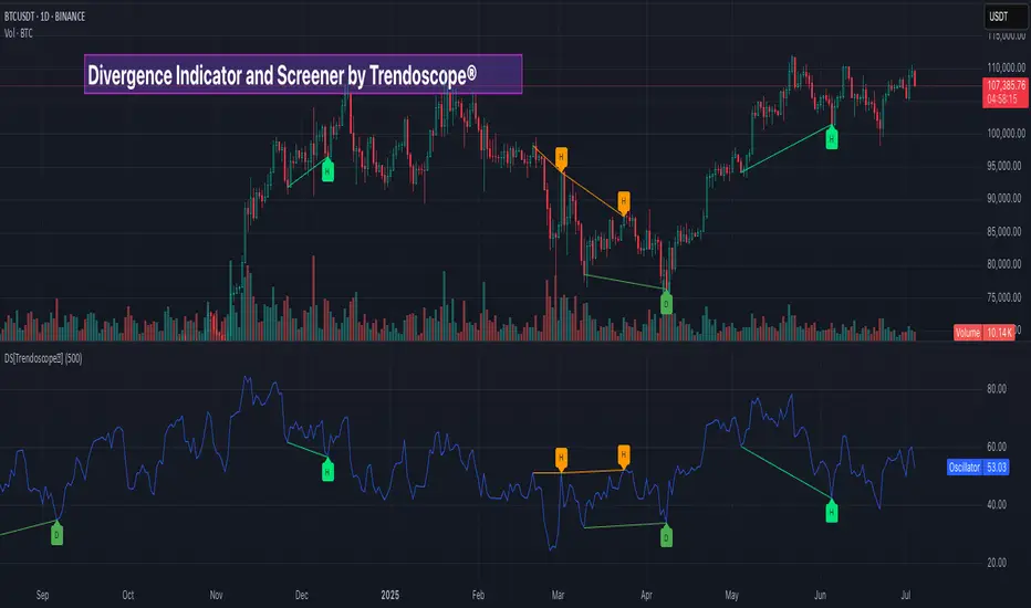
Divergence Screener [Trendoscope®]🎲Overview
The Divergence Screener is a powerful TradingView indicator designed to detect and visualize bullish and bearish divergences, including hidden divergences, between price action and a user-selected oscillator. Built with flexibility in mind, it allows traders to customize the oscillator type, trend detection method, and other parameters to suit various trading strategies. The indicator is non-overlay, displaying divergence signals directly on the oscillator plot, with visual cues such as lines and labels on the chart for easy identification.
This indicator is ideal for traders seeking to identify potential reversal or continuation signals based on price-oscillator divergences. It supports multiple oscillators, trend detection methods, and alert configurations, making it versatile for different markets and timeframes.
🎲Features
🎯Customizable Oscillator Selection
Built-in Oscillators : Choose from a variety of oscillators including RSI, CCI, CMO, COG, MFI, ROC, Stochastic, and WPR.
External Oscillator Support : Users can input an external oscillator source, allowing integration with custom or third-party indicators.
Configurable Length : Adjust the oscillator’s period (e.g., 14 for RSI) to fine-tune sensitivity.
🎯Divergence Detection
The screener identifies four types of divergences:
Bullish Divergence : Price forms a lower low, but the oscillator forms a higher low, signaling potential upward reversal.
Bearish Divergence : Price forms a higher high, but the oscillator forms a lower high, indicating potential downward reversal.
Bullish Hidden Divergence : Price forms a higher low, but the oscillator forms a lower low, suggesting trend continuation in an uptrend.
Bearish Hidden Divergence : Price forms a lower high, but the oscillator forms a higher high, suggesting trend continuation in a downtrend.
🎯Flexible Trend Detection
The indicator offers three methods to determine the trend context for divergence detection:
Zigzag : Uses zigzag pivots to identify trends based on higher highs (HH), higher lows (HL), lower highs (LH), and lower lows (LL).
MA Difference : Calculates the trend based on the difference in a moving average (e.g., SMA, EMA) between divergence pivots.
External Trend Signal : Allows users to input an external trend signal (positive for uptrend, negative for downtrend) for custom trend analysis.
🎯Zigzag-Based Pivot Analysis
Customizable Zigzag Length : Adjust the zigzag length (default: 13) to control the sensitivity of pivot detection.
Repaint Option : Choose whether divergence lines repaint based on the latest data or wait for confirmed pivots, balancing responsiveness and reliability.
🎯Visual and Alert Features
Divergence Visualization : Divergence lines are drawn between price pivots and oscillator pivots, color-coded for easy identification:
Bullish Divergence : Green
Bearish Divergence : Red
Bullish Hidden Divergence : Lime
Bearish Hidden Divergence : Orange
Labels and Tooltips : Labels (e.g., “D” for divergence, “H” for hidden) appear on price and oscillator pivots, with tooltips providing detailed information such as price/oscillator values, ratios, and pivot directions.
Alerts : Configurable alerts for each divergence type (bullish, bearish, bullish hidden, bearish hidden) trigger on bar close, ensuring timely notifications.
🎲 How It Works
🎯Oscillator Calculation
The indicator calculates the selected oscillator (or uses an external source) and plots it on the chart.
Oscillator values are stored in a map for reference during divergence calculations.
🎯Pivot Detection
A zigzag algorithm identifies pivots in the oscillator data, with configurable length and repainting options.
Price and oscillator pivots are compared to detect divergences based on their direction and ratio.
🎯Divergence Identification
The indicator compares price and oscillator pivot directions (HH, HL, LH, LL) to identify divergences.
Trend context is determined using the selected method (Zigzag, MA Difference, or External).
Divergences are classified as bullish, bearish, bullish hidden, or bearish hidden based on price-oscillator relationships and trend direction.
🎯Visualization and Alerts
Valid divergences are drawn as lines connecting price and oscillator pivots, with corresponding labels.
Alerts are triggered for allowed divergence types, providing detailed information via tooltips.
🎯Validation
Divergence lines are validated to ensure no intermediate bars violate the divergence condition, enhancing signal reliability.
🎲 Usage Instructions as Indicator
🎯Add to Chart:
Add the “Divergence Screener ” to your TradingView chart.
The indicator appears in a separate pane below the price chart, plotting the oscillator and divergence signals.
🎯Configure Settings:
Adjust the oscillator type and length to match your trading style.
Select a trend detection method and configure related parameters (e.g., MA type/length or external signal).
Set the zigzag length and repainting preference.
Enable/disable alerts for specific divergence types.
I🎯nterpret Signals:
Bullish Divergence (Green) : Look for potential buy opportunities in a downtrend.
Bearish Divergence (Red) : Consider sell opportunities in an uptrend.
Bullish Hidden Divergence (Lime) : Confirm continuation in an uptrend.
Bearish Hidden Divergence (Orange): Confirm continuation in a downtrend.
Use tooltips on labels to review detailed pivot and divergence information.
🎯Set Alerts:
Create alerts for each divergence type to receive notifications via TradingView’s alert system.
Alerts include detailed text with price, oscillator, and divergence information.
🎲 Example Scenarios as Indicator
🎯 With External Oscillator (Use MACD Histogram as Oscillator)
In order to use MACD as an oscillator for divergence signal instead of the built in options, follow these steps.
Load MACD Indicator from Indicator library
From Indicator settings of Divergence Screener, set Use External Oscillator and select MACD Histograme from the dropdown
You can now see that the oscillator pane shows the data of selected MACD histogram and divergence signals are generated based on the external MACD histogram data.
🎯 With External Trend Signal (Supertrend Ladder ATR)
Now let's demonstrate how to use external direction signals using Supertrend Ladder ATR indicator. Please note that in order to use the indicator as trend source, the indicator should return positive integer for uptrend and negative integer for downtrend. Steps are as follows:
Load the desired trend indicator. In this example, we are using Supertrend Ladder ATR
From the settings of Divergence Screener, select "External" as Trend Detection Method
Select the trend detection plot Direction from the dropdown. You can now see that the divergence signals will rely on the new trend settings rather than the built in options.
🎲 Using the Script with Pine Screener
The primary purpose of the Divergence Screener is to enable traders to scan multiple instruments (e.g., stocks, ETFs, forex pairs) for divergence signals using TradingView’s Pine Screener, facilitating efficient comparison and identification of trading opportunities.
To use the Divergence Screener as a screener, follow these steps:
Add to Favorites : Add the Divergence Screener to your TradingView favorites to make it available in the Pine Screener.
Create a Watchlist : Build a watchlist containing the instruments (e.g., stocks, ETFs, or forex pairs) you want to scan for divergences.
Access Pine Screener : Navigate to the Pine Screener via TradingView’s main menu: Products -> Screeners -> Pine, or directly visit tradingview.com/pine-screener/.
Select Watchlist : Choose the watchlist you created from the Watchlist dropdown in the Pine Screener interface.
Choose Indicator : Select Divergence Screener from the Choose Indicator dropdown.
Configure Settings : Set the desired timeframe (e.g., 1 hour, 1 day) and adjust indicator settings such as oscillator type, zigzag length, or trend detection method as needed.
Select Filter Criteria : Select the condition on which the watchlist items needs to be filtered. Filtering can only be done on the plots defined in the script.
Run Scan : Press the Scan button to display divergence signals across the selected instruments. The screener will show which instruments exhibit bullish, bearish, bullish hidden, or bearish hidden divergences based on the configured settings.
🎲 Limitations and Possible Future Enhancements
Limitations are
Custom input for oscillator and trend detection cannot be used in pine screener.
Pine screener has max 500 bars available.
Repaint option is by default enabled. When in repaint mode expect the early signal but the signals are prone to repaint.
Possible future enhancements
Add more built-in options for oscillators and trend detection methods so that dependency on external indicators is limited
Multi level zigzag support
log.info() - 5 Exampleslog.info() is one of the most powerful tools in Pine Script that no one knows about. Whenever you code, you want to be able to debug, or find out why something isn’t working. The log.info() command will help you do that. Without it, creating more complex Pine Scripts becomes exponentially more difficult.
The first thing to note is that log.info() only displays strings. So, if you have a variable that is not a string, you must turn it into a string in order for log.info() to work. The way you do that is with the str.tostring() command. And remember, it's all lower case! You can throw in any numeric value (float, int, timestamp) into str.string() and it should work.
Next, in order to make your output intelligible, you may want to identify whatever value you are logging. For example, if an RSI value is 50, you don’t want a bunch of lines that just say “50”. You may want it to say “RSI = 50”.
To do that, you’ll have to use the concatenation operator. For example, if you have a variable called “rsi”, and its value is 50, then you would use the “+” concatenation symbol.
EXAMPLE 1
━━━━━━━━━━━━━━━━━━━━━━━━━━━━━━━━━
//@version=6
indicator("log.info()")
rsi = ta.rsi(close,14)
log.info(“RSI= ” + str.tostring(rsi))
Example Output =>
RSI= 50
Here, we use double quotes to create a string that contains the name of the variable, in this case “RSI = “, then we concatenate it with a stringified version of the variable, rsi.
Now that you know how to write a log, where do you view them? There isn’t a lot of documentation on it, and the link is not conveniently located.
Open up the “Pine Editor” tab at the bottom of any chart view, and you’ll see a “3 dot” button at the top right of the pane. Click that, and right above the “Help” menu item you’ll see “Pine logs”. Clicking that will open that to open a pane on the right of your browser - replacing whatever was in the right pane area before. This is where your log output will show up.
But, because you’re dealing with time series data, using the log.info() command without some type of condition will give you a fast moving stream of numbers that will be difficult to interpret. So, you may only want the output to show up once per bar, or only under specific conditions.
To have the output show up only after all computations have completed, you’ll need to use the barState.islast command. Remember, barState is camelCase, but islast is not!
EXAMPLE 2
━━━━━━━━━━━━━━━━━━━━━━━━━━━━━━━━━
//@version=6
indicator("log.info()")
rsi = ta.rsi(close,14)
if barState.islast
log.info("RSI=" + str.tostring(rsi))
plot(rsi)
However, this can be less than ideal, because you may want the value of the rsi variable on a particular bar, at a particular time, or under a specific chart condition. Let’s hit these one at a time.
In each of these cases, the built-in bar_index variable will come in handy. When debugging, I typically like to assign a variable “bix” to represent bar_index, and include it in the output.
So, if I want to see the rsi value when RSI crosses above 0.5, then I would have something like
EXAMPLE 3
━━━━━━━━━━━━━━━━━━━━━━━━━━━━━━━━━
//@version=6
indicator("log.info()")
rsi = ta.rsi(close,14)
bix = bar_index
rsiCrossedOver = ta.crossover(rsi,0.5)
if rsiCrossedOver
log.info("bix=" + str.tostring(bix) + " - RSI=" + str.tostring(rsi))
plot(rsi)
Example Output =>
bix=19964 - RSI=51.8449459867
bix=19972 - RSI=50.0975830828
bix=19983 - RSI=53.3529808079
bix=19985 - RSI=53.1595745146
bix=19999 - RSI=66.6466337654
bix=20001 - RSI=52.2191767466
Here, we see that the output only appears when the condition is met.
A useful thing to know is that if you want to limit the number of decimal places, then you would use the command str.tostring(rsi,”#.##”), which tells the interpreter that the format of the number should only be 2 decimal places. Or you could round the rsi variable with a command like rsi2 = math.round(rsi*100)/100 . In either case you’re output would look like:
bix=19964 - RSI=51.84
bix=19972 - RSI=50.1
bix=19983 - RSI=53.35
bix=19985 - RSI=53.16
bix=19999 - RSI=66.65
bix=20001 - RSI=52.22
This would decrease the amount of memory that’s being used to display your variable’s values, which can become a limitation for the log.info() command. It only allows 4096 characters per line, so when you get to trying to output arrays (which is another cool feature), you’ll have to keep that in mind.
Another thing to note is that log output is always preceded by a timestamp, but for the sake of brevity, I’m not including those in the output examples.
If you wanted to only output a value after the chart was fully loaded, that’s when barState.islast command comes in. Under this condition, only one line of output is created per tick update — AFTER the chart has finished loading. For example, if you only want to see what the the current bar_index and rsi values are, without filling up your log window with everything that happens before, then you could use the following code:
EXAMPLE 4
━━━━━━━━━━━━━━━━━━━━━━━━━━━━━━━━━
//@version=6
indicator("log.info()")
rsi = ta.rsi(close,14)
bix = bar_index
if barstate.islast
log.info("bix=" + str.tostring(bix) + " - RSI=" + str.tostring(rsi))
Example Output =>
bix=20203 - RSI=53.1103309071
This value would keep updating after every new bar tick.
The log.info() command is a huge help in creating new scripts, however, it does have its limitations. As mentioned earlier, only 4096 characters are allowed per line. So, although you can use log.info() to output arrays, you have to be aware of how many characters that array will use.
The following code DOES NOT WORK! And, the only way you can find out why will be the red exclamation point next to the name of the indicator. That, and nothing will show up on the chart, or in the logs.
// CODE DOESN’T WORK
//@version=6
indicator("MW - log.info()")
var array rsi_arr = array.new()
rsi = ta.rsi(close,14)
bix = bar_index
rsiCrossedOver = ta.crossover(rsi,50)
if rsiCrossedOver
array.push(rsi_arr, rsi)
if barstate.islast
log.info("rsi_arr:" + str.tostring(rsi_arr))
log.info("bix=" + str.tostring(bix) + " - RSI=" + str.tostring(rsi))
plot(rsi)
// No code errors, but will not compile because too much is being written to the logs.
However, after putting some time restrictions in with the i_startTime and i_endTime user input variables, and creating a dateFilter variable to use in the conditions, I can limit the size of the final array. So, the following code does work.
EXAMPLE 5
━━━━━━━━━━━━━━━━━━━━━━━━━━━━━━━━━
// CODE DOES WORK
//@version=6
indicator("MW - log.info()")
i_startTime = input.time(title="Start", defval=timestamp("01 Jan 2025 13:30 +0000"))
i_endTime = input.time(title="End", defval=timestamp("1 Jan 2099 19:30 +0000"))
var array rsi_arr = array.new()
dateFilter = time >= i_startTime and time <= i_endTime
rsi = ta.rsi(close,14)
bix = bar_index
rsiCrossedOver = ta.crossover(rsi,50) and dateFilter // <== The dateFilter condition keeps the array from getting too big
if rsiCrossedOver
array.push(rsi_arr, rsi)
if barstate.islast
log.info("rsi_arr:" + str.tostring(rsi_arr))
log.info("bix=" + str.tostring(bix) + " - RSI=" + str.tostring(rsi))
plot(rsi)
Example Output =>
rsi_arr:
bix=20210 - RSI=56.9030578034
Of course, if you restrict the decimal places by using the rounding the rsi value with something like rsiRounded = math.round(rsi * 100) / 100 , then you can further reduce the size of your array. In this case the output may look something like:
Example Output =>
rsi_arr:
bix=20210 - RSI=55.6947486019
This will give your code a little breathing room.
In a nutshell, I was coding for over a year trying to debug by pushing output to labels, tables, and using libraries that cluttered up my code. Once I was able to debug with log.info() it was a game changer. I was able to start building much more advanced scripts. Hopefully, this will help you on your journey as well.

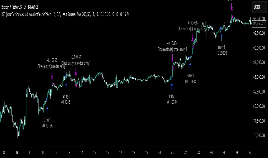
KST Strategy [Skyrexio]Overview
KST Strategy leverages Know Sure Thing (KST) indicator in conjunction with the Williams Alligator and Moving average to obtain the high probability setups. KST is used for for having the high probability to enter in the direction of a current trend when momentum is rising, Alligator is used as a short term trend filter, while Moving average approximates the long term trend and allows trades only in its direction. Also strategy has the additional optional filter on Choppiness Index which does not allow trades if market is choppy, above the user-specified threshold. Strategy has the user specified take profit and stop-loss numbers, but multiplied by Average True Range (ATR) value on the moment when trade is open. The strategy opens only long trades.
Unique Features
ATR based stop-loss and take profit. Instead of fixed take profit and stop-loss percentage strategy utilizes user chosen numbers multiplied by ATR for its calculation.
Configurable Trading Periods. Users can tailor the strategy to specific market windows, adapting to different market conditions.
Optional Choppiness Index filter. Strategy allows to choose if it will use the filter trades with Choppiness Index and set up its threshold.
Methodology
The strategy opens long trade when the following price met the conditions:
Close price is above the Alligator's jaw line
Close price is above the filtering Moving average
KST line of Know Sure Thing indicator shall cross over its signal line (details in justification of methodology)
If the Choppiness Index filter is enabled its value shall be less than user defined threshold
When the long trade is executed algorithm defines the stop-loss level as the low minus user defined number, multiplied by ATR at the trade open candle. Also it defines take profit with close price plus user defined number, multiplied by ATR at the trade open candle. While trade is in progress, if high price on any candle above the calculated take profit level or low price is below the calculated stop loss level, trade is closed.
Strategy settings
In the inputs window user can setup the following strategy settings:
ATR Stop Loss (by default = 1.5, number of ATRs to calculate stop-loss level)
ATR Take Profit (by default = 3.5, number of ATRs to calculate take profit level)
Filter MA Type (by default = Least Squares MA, type of moving average which is used for filter MA)
Filter MA Length (by default = 200, length for filter MA calculation)
Enable Choppiness Index Filter (by default = true, setting to choose the optional filtering using Choppiness index)
Choppiness Index Threshold (by default = 50, Choppiness Index threshold, its value shall be below it to allow trades execution)
Choppiness Index Length (by default = 14, length used in Choppiness index calculation)
KST ROC Length #1 (by default = 10, value used in KST indicator calculation, more information in Justification of Methodology)
KST ROC Length #2 (by default = 15, value used in KST indicator calculation, more information in Justification of Methodology)
KST ROC Length #3 (by default = 20, value used in KST indicator calculation, more information in Justification of Methodology)
KST ROC Length #4 (by default = 30, value used in KST indicator calculation, more information in Justification of Methodology)
KST SMA Length #1 (by default = 10, value used in KST indicator calculation, more information in Justification of Methodology)
KST SMA Length #2 (by default = 10, value used in KST indicator calculation, more information in Justification of Methodology)
KST SMA Length #3 (by default = 10, value used in KST indicator calculation, more information in Justification of Methodology)
KST SMA Length #4 (by default = 15, value used in KST indicator calculation, more information in Justification of Methodology)
KST Signal Line Length (by default = 10, value used in KST indicator calculation, more information in Justification of Methodology)
User can choose the optimal parameters during backtesting on certain price chart.
Justification of Methodology
Before understanding why this particular combination of indicator has been chosen let's briefly explain what is KST, Williams Alligator, Moving Average, ATR and Choppiness Index.
The KST (Know Sure Thing) is a momentum oscillator developed by Martin Pring. It combines multiple Rate of Change (ROC) values, smoothed over different timeframes, to identify trend direction and momentum strength. First of all, what is ROC? ROC (Rate of Change) is a momentum indicator that measures the percentage change in price between the current price and the price a set number of periods ago.
ROC = 100 * (Current Price - Price N Periods Ago) / Price N Periods Ago
In our case N is the KST ROC Length inputs from settings, here we will calculate 4 different ROCs to obtain KST value:
KST = ROC1_smooth × 1 + ROC2_smooth × 2 + ROC3_smooth × 3 + ROC4_smooth × 4
ROC1 = ROC(close, KST ROC Length #1), smoothed by KST SMA Length #1,
ROC2 = ROC(close, KST ROC Length #2), smoothed by KST SMA Length #2,
ROC3 = ROC(close, KST ROC Length #3), smoothed by KST SMA Length #3,
ROC4 = ROC(close, KST ROC Length #4), smoothed by KST SMA Length #4
Also for this indicator the signal line is calculated:
Signal = SMA(KST, KST Signal Line Length)
When the KST line rises, it indicates increasing momentum and suggests that an upward trend may be developing. Conversely, when the KST line declines, it reflects weakening momentum and a potential downward trend. A crossover of the KST line above its signal line is considered a buy signal, while a crossover below the signal line is viewed as a sell signal. If the KST stays above zero, it indicates overall bullish momentum; if it remains below zero, it points to bearish momentum. The KST indicator smooths momentum across multiple timeframes, helping to reduce noise and provide clearer signals for medium- to long-term trends.
Next, let’s discuss the short-term trend filter, which combines the Williams Alligator and Williams Fractals. Williams Alligator
Developed by Bill Williams, the Alligator is a technical indicator that identifies trends and potential market reversals. It consists of three smoothed moving averages:
Jaw (Blue Line): The slowest of the three, based on a 13-period smoothed moving average shifted 8 bars ahead.
Teeth (Red Line): The medium-speed line, derived from an 8-period smoothed moving average shifted 5 bars forward.
Lips (Green Line): The fastest line, calculated using a 5-period smoothed moving average shifted 3 bars forward.
When the lines diverge and align in order, the "Alligator" is "awake," signaling a strong trend. When the lines overlap or intertwine, the "Alligator" is "asleep," indicating a range-bound or sideways market. This indicator helps traders determine when to enter or avoid trades.
The next indicator is Moving Average. It has a lot of different types which can be chosen to filter trades and the Least Squares MA is used by default settings. Let's briefly explain what is it.
The Least Squares Moving Average (LSMA) — also known as Linear Regression Moving Average — is a trend-following indicator that uses the least squares method to fit a straight line to the price data over a given period, then plots the value of that line at the most recent point. It draws the best-fitting straight line through the past N prices (using linear regression), and then takes the endpoint of that line as the value of the moving average for that bar. The LSMA aims to reduce lag and highlight the current trend more accurately than traditional moving averages like SMA or EMA.
Key Features:
It reacts faster to price changes than most moving averages.
It is smoother and less noisy than short-term EMAs.
It can be used to identify trend direction, momentum, and potential reversal points.
ATR (Average True Range) is a volatility indicator that measures how much an asset typically moves during a given period. It was introduced by J. Welles Wilder and is widely used to assess market volatility, not direction.
To calculate it first of all we need to get True Range (TR), this is the greatest value among:
High - Low
abs(High - Previous Close)
abs(Low - Previous Close)
ATR = MA(TR, n) , where n is number of periods for moving average, in our case equals 14.
ATR shows how much an asset moves on average per candle/bar. A higher ATR means more volatility; a lower ATR means a calmer market.
The Choppiness Index is a technical indicator that quantifies whether the market is trending or choppy (sideways). It doesn't indicate trend direction — only the strength or weakness of a trend. Higher Choppiness Index usually approximates the sideways market, while its low value tells us that there is a high probability of a trend.
Choppiness Index = 100 × log10(ΣATR(n) / (MaxHigh(n) - MinLow(n))) / log10(n)
where:
ΣATR(n) = sum of the Average True Range over n periods
MaxHigh(n) = highest high over n periods
MinLow(n) = lowest low over n periods
log10 = base-10 logarithm
Now let's understand how these indicators work in conjunction and why they were chosen for this strategy. KST indicator approximates current momentum, when it is rising and KST line crosses over the signal line there is high probability that short term trend is reversing to the upside and strategy allows to take part in this potential move. Alligator's jaw (blue) line is used as an approximation of a short term trend, taking trades only above it we want to avoid trading against trend to increase probability that long trade is going to be winning.
Almost the same for Moving Average, but it approximates the long term trend, this is just the additional filter. If we trade in the direction of the long term trend we increase probability that higher risk to reward trade will hit the take profit. Choppiness index is the optional filter, but if it turned on it is used for approximating if now market is in sideways or in trend. On the range bounded market the potential moves are restricted. We want to decrease probability opening trades in such condition avoiding trades if this index is above threshold value.
When trade is open script sets the stop loss and take profit targets. ATR approximates the current volatility, so we can make a decision when to exit a trade based on current market condition, it can increase the probability that strategy will avoid the excessive stop loss hits, but anyway user can setup how many ATRs to use as a stop loss and take profit target. As was said in the Methodology stop loss level is obtained by subtracting number of ATRs from trade opening candle low, while take profit by adding to this candle's close.
Backtest Results
Operating window: Date range of backtests is 2023.01.01 - 2025.05.01. It is chosen to let the strategy to close all opened positions.
Commission and Slippage: Includes a standard Binance commission of 0.1% and accounts for possible slippage over 5 ticks.
Initial capital: 10000 USDT
Percent of capital used in every trade: 60%
Maximum Single Position Loss: -5.53%
Maximum Single Profit: +8.35%
Net Profit: +5175.20 USDT (+51.75%)
Total Trades: 120 (56.67% win rate)
Profit Factor: 1.747
Maximum Accumulated Loss: 1039.89 USDT (-9.1%)
Average Profit per Trade: 43.13 USDT (+0.6%)
Average Trade Duration: 27 hours
These results are obtained with realistic parameters representing trading conditions observed at major exchanges such as Binance and with realistic trading portfolio usage parameters.
How to Use
Add the script to favorites for easy access.
Apply to the desired timeframe and chart (optimal performance observed on 1h BTC/USDT).
Configure settings using the dropdown choice list in the built-in menu.
Set up alerts to automate strategy positions through web hook with the text: {{strategy.order.alert_message}}
Disclaimer:
Educational and informational tool reflecting Skyrexio commitment to informed trading. Past performance does not guarantee future results. Test strategies in a simulated environment before live implementation.
LVN/HVN Auto Detection [PhenLabs]📊 PhenLabs - LVN/HVN Auto Detection
Version: PineScript™ v6
📌 Description
The PhenLabs LVN/HVN Auto Detection indicator is an advanced volume profile analysis tool that automatically identifies Low Volume Nodes (LVN) and High Volume Nodes (HVN) across multiple trading sessions. This sophisticated indicator analyzes volume distribution patterns to pinpoint critical support and resistance levels where price is likely to react, providing traders with high-probability zones for entries, exits, and risk management.
Unlike traditional volume indicators that only show current activity, this tool builds comprehensive volume profiles from historical sessions and intelligently filters the most significant levels. It combines real-time volume analysis with dynamic level detection, offering both visual bubbles for immediate volume activity and persistent horizontal lines that act as ongoing support/resistance references.
🚀 Points of Innovation
Multi-Session Volume Profile Analysis - Automatically calculates and analyzes volume profiles across the last 5 trading sessions
Intelligent Level Separation Logic - Prevents overlapping signals by maintaining minimum separation between LVN and HVN levels
Dynamic Timeframe Adaptation - Automatically adjusts session lengths based on chart timeframe for optimal level detection
Real-Time Activity Bubbles - Shows volume activity strength through different bubble sizes at key levels
Persistent Line Management - Creates horizontal lines that extend until price crosses them, providing ongoing reference points
Dual Threshold System - Independent percentage-based thresholds for both LVN and HVN identification
🔧 Core Components
Volume Profile Engine : Builds 20-row volume profiles for each analyzed session, distributing volume across price levels
Level Identification Algorithm : Uses percentage-based thresholds to classify volume distribution patterns
Separation Logic : Ensures minimum distance between conflicting levels, prioritizing HVN when overlap occurs
Line Management System : Tracks active support/resistance lines and removes them when price crosses through
Volume Activity Monitor : Compares current volume to 13-period moving average for activity classification
🔥 Key Features
Customizable Thresholds : LVN threshold (5-35%, default 20%) and HVN threshold (65-95%, default 80%) for precise level filtering
Volume Activity Multiplier : Adjustable volume threshold (0.5+, default 1.5) for bubble and line creation sensitivity
Flexible Display Modes : Choose between Lines only, Bubbles only, or Both for optimal chart clarity
Smart Level Separation : Minimum separation percentage (0.1-2%, default 0.5%) prevents conflicting signals
Color Customization : Independent color controls for LVN (red) and HVN (blue) elements
Performance Optimization : Processes every 15 bars with maximum 500 active lines for smooth operation
🎨 Visualization
Colored Bubbles : Three sizes (large, medium, small) indicate volume activity strength at key levels
Horizontal Lines : Persistent support/resistance lines with width corresponding to volume activity
Dual Color System : Semi-transparent red for LVN areas, semi-transparent blue for HVN zones
Information Tooltip : Optional table showing usage guidelines and optimization tips
📖 Usage Guidelines
Volume Thresholds
LVN Threshold
○ Default: 20.0%
○ Range: 5.0-35.0%
○ Description: Price levels with volume below this percentage are marked as LVNs. Lower values create fewer, more significant levels. Typical range 15-25% works for most instruments.
HVN Threshold
○ Default: 80.0%
○ Range: 65.0-95.0%
○ Description: Price levels with volume above this percentage are marked as HVNs. Higher values create fewer, stronger levels. Range 75-85% is optimal for most trading.
Display Controls
Volume Threshold
○ Default: 1.5
○ Range: 0.5+
○ Description: Multiplier for volume significance (High=2+threshold, Medium=1+threshold, Low=0+threshold). Higher values require more volume for signals.
✅ Best Use Cases
Swing Trading : Identify key levels for position entries and exits over multiple days
Scalping : Use bubbles for immediate volume activity confirmation at critical levels
Risk Management : Place stops beyond LVN levels where price moves quickly
Breakout Trading : Monitor HVN levels for potential breakout or rejection scenarios
Multi-Timeframe Analysis : Combine with higher timeframe levels for confluence
⚠️ Limitations
Timeframe Sensitivity : Lower timeframes may produce too many levels; higher timeframes recommended for cleaner signals
Volume Data Dependency : Accuracy depends on reliable volume data from your data provider
Historical Analysis : Uses past volume data which may not predict future price behavior
Performance Impact : High number of active lines may affect chart performance on slower devices
💡 What Makes This Unique
Automated Session Analysis : No manual drawing required - automatically analyzes multiple sessions
Intelligent Filtering : Advanced separation logic prevents overlapping and conflicting signals
Adaptive Processing : Adjusts to different timeframes automatically for optimal level detection
Dual Visualization System : Combines persistent lines with real-time activity indicators
🔬 How It Works
1. Volume Profile Construction :
Analyzes the last 5 trading sessions with dynamic session length based on timeframe
Divides each session’s price range into 20 equal levels for volume distribution analysis
2. Level Classification :
Calculates volume percentage at each price level relative to session maximum
Identifies LVN levels below threshold and HVN levels above threshold
3. Signal Generation :
Creates bubbles when volume activity exceeds thresholds at identified levels
Draws horizontal lines that persist until price crosses through them
💡 Note : For optimal results, increase your chart timeframe if you see too many levels. The indicator performs best on 15-minute and higher timeframes where volume patterns are more meaningful and less noisy.

Tensor Market Analysis Engine (TMAE)# Tensor Market Analysis Engine (TMAE)
## Advanced Multi-Dimensional Mathematical Analysis System
*Where Quantum Mathematics Meets Market Structure*
---
## 🎓 THEORETICAL FOUNDATION
The Tensor Market Analysis Engine represents a revolutionary synthesis of three cutting-edge mathematical frameworks that have never before been combined for comprehensive market analysis. This indicator transcends traditional technical analysis by implementing advanced mathematical concepts from quantum mechanics, information theory, and fractal geometry.
### 🌊 Multi-Dimensional Volatility with Jump Detection
**Hawkes Process Implementation:**
The TMAE employs a sophisticated Hawkes process approximation for detecting self-exciting market jumps. Unlike traditional volatility measures that treat price movements as independent events, the Hawkes process recognizes that market shocks cluster and exhibit memory effects.
**Mathematical Foundation:**
```
Intensity λ(t) = μ + Σ α(t - Tᵢ)
```
Where market jumps at times Tᵢ increase the probability of future jumps through the decay function α, controlled by the Hawkes Decay parameter (0.5-0.99).
**Mahalanobis Distance Calculation:**
The engine calculates volatility jumps using multi-dimensional Mahalanobis distance across up to 5 volatility dimensions:
- **Dimension 1:** Price volatility (standard deviation of returns)
- **Dimension 2:** Volume volatility (normalized volume fluctuations)
- **Dimension 3:** Range volatility (high-low spread variations)
- **Dimension 4:** Correlation volatility (price-volume relationship changes)
- **Dimension 5:** Microstructure volatility (intrabar positioning analysis)
This creates a volatility state vector that captures market behavior impossible to detect with traditional single-dimensional approaches.
### 📐 Hurst Exponent Regime Detection
**Fractal Market Hypothesis Integration:**
The TMAE implements advanced Rescaled Range (R/S) analysis to calculate the Hurst exponent in real-time, providing dynamic regime classification:
- **H > 0.6:** Trending (persistent) markets - momentum strategies optimal
- **H < 0.4:** Mean-reverting (anti-persistent) markets - contrarian strategies optimal
- **H ≈ 0.5:** Random walk markets - breakout strategies preferred
**Adaptive R/S Analysis:**
Unlike static implementations, the TMAE uses adaptive windowing that adjusts to market conditions:
```
H = log(R/S) / log(n)
```
Where R is the range of cumulative deviations and S is the standard deviation over period n.
**Dynamic Regime Classification:**
The system employs hysteresis to prevent regime flipping, requiring sustained Hurst values before regime changes are confirmed. This prevents false signals during transitional periods.
### 🔄 Transfer Entropy Analysis
**Information Flow Quantification:**
Transfer entropy measures the directional flow of information between price and volume, revealing lead-lag relationships that indicate future price movements:
```
TE(X→Y) = Σ p(yₜ₊₁, yₜ, xₜ) log
```
**Causality Detection:**
- **Volume → Price:** Indicates accumulation/distribution phases
- **Price → Volume:** Suggests retail participation or momentum chasing
- **Balanced Flow:** Market equilibrium or transition periods
The system analyzes multiple lag periods (2-20 bars) to capture both immediate and structural information flows.
---
## 🔧 COMPREHENSIVE INPUT SYSTEM
### Core Parameters Group
**Primary Analysis Window (10-100, Default: 50)**
The fundamental lookback period affecting all calculations. Optimization by timeframe:
- **1-5 minute charts:** 20-30 (rapid adaptation to micro-movements)
- **15 minute-1 hour:** 30-50 (balanced responsiveness and stability)
- **4 hour-daily:** 50-100 (smooth signals, reduced noise)
- **Asset-specific:** Cryptocurrency 20-35, Stocks 35-50, Forex 40-60
**Signal Sensitivity (0.1-2.0, Default: 0.7)**
Master control affecting all threshold calculations:
- **Conservative (0.3-0.6):** High-quality signals only, fewer false positives
- **Balanced (0.7-1.0):** Optimal risk-reward ratio for most trading styles
- **Aggressive (1.1-2.0):** Maximum signal frequency, requires careful filtering
**Signal Generation Mode:**
- **Aggressive:** Any component signals (highest frequency)
- **Confluence:** 2+ components agree (balanced approach)
- **Conservative:** All 3 components align (highest quality)
### Volatility Jump Detection Group
**Volatility Dimensions (2-5, Default: 3)**
Determines the mathematical space complexity:
- **2D:** Price + Volume volatility (suitable for clean markets)
- **3D:** + Range volatility (optimal for most conditions)
- **4D:** + Correlation volatility (advanced multi-asset analysis)
- **5D:** + Microstructure volatility (maximum sensitivity)
**Jump Detection Threshold (1.5-4.0σ, Default: 3.0σ)**
Standard deviations required for volatility jump classification:
- **Cryptocurrency:** 2.0-2.5σ (naturally volatile)
- **Stock Indices:** 2.5-3.0σ (moderate volatility)
- **Forex Major Pairs:** 3.0-3.5σ (typically stable)
- **Commodities:** 2.0-3.0σ (varies by commodity)
**Jump Clustering Decay (0.5-0.99, Default: 0.85)**
Hawkes process memory parameter:
- **0.5-0.7:** Fast decay (jumps treated as independent)
- **0.8-0.9:** Moderate clustering (realistic market behavior)
- **0.95-0.99:** Strong clustering (crisis/event-driven markets)
### Hurst Exponent Analysis Group
**Calculation Method Options:**
- **Classic R/S:** Original Rescaled Range (fast, simple)
- **Adaptive R/S:** Dynamic windowing (recommended for trading)
- **DFA:** Detrended Fluctuation Analysis (best for noisy data)
**Trending Threshold (0.55-0.8, Default: 0.60)**
Hurst value defining persistent market behavior:
- **0.55-0.60:** Weak trend persistence
- **0.65-0.70:** Clear trending behavior
- **0.75-0.80:** Strong momentum regimes
**Mean Reversion Threshold (0.2-0.45, Default: 0.40)**
Hurst value defining anti-persistent behavior:
- **0.35-0.45:** Weak mean reversion
- **0.25-0.35:** Clear ranging behavior
- **0.15-0.25:** Strong reversion tendency
### Transfer Entropy Parameters Group
**Information Flow Analysis:**
- **Price-Volume:** Classic flow analysis for accumulation/distribution
- **Price-Volatility:** Risk flow analysis for sentiment shifts
- **Multi-Timeframe:** Cross-timeframe causality detection
**Maximum Lag (2-20, Default: 5)**
Causality detection window:
- **2-5 bars:** Immediate causality (scalping)
- **5-10 bars:** Short-term flow (day trading)
- **10-20 bars:** Structural flow (swing trading)
**Significance Threshold (0.05-0.3, Default: 0.15)**
Minimum entropy for signal generation:
- **0.05-0.10:** Detect subtle information flows
- **0.10-0.20:** Clear causality only
- **0.20-0.30:** Very strong flows only
---
## 🎨 ADVANCED VISUAL SYSTEM
### Tensor Volatility Field Visualization
**Five-Layer Resonance Bands:**
The tensor field creates dynamic support/resistance zones that expand and contract based on mathematical field strength:
- **Core Layer (Purple):** Primary tensor field with highest intensity
- **Layer 2 (Neutral):** Secondary mathematical resonance
- **Layer 3 (Info Blue):** Tertiary harmonic frequencies
- **Layer 4 (Warning Gold):** Outer field boundaries
- **Layer 5 (Success Green):** Maximum field extension
**Field Strength Calculation:**
```
Field Strength = min(3.0, Mahalanobis Distance × Tensor Intensity)
```
The field amplitude adjusts to ATR and mathematical distance, creating dynamic zones that respond to market volatility.
**Radiation Line Network:**
During active tensor states, the system projects directional radiation lines showing field energy distribution:
- **8 Directional Rays:** Complete angular coverage
- **Tapering Segments:** Progressive transparency for natural visual flow
- **Pulse Effects:** Enhanced visualization during volatility jumps
### Dimensional Portal System
**Portal Mathematics:**
Dimensional portals visualize regime transitions using category theory principles:
- **Green Portals (◉):** Trending regime detection (appear below price for support)
- **Red Portals (◎):** Mean-reverting regime (appear above price for resistance)
- **Yellow Portals (○):** Random walk regime (neutral positioning)
**Tensor Trail Effects:**
Each portal generates 8 trailing particles showing mathematical momentum:
- **Large Particles (●):** Strong mathematical signal
- **Medium Particles (◦):** Moderate signal strength
- **Small Particles (·):** Weak signal continuation
- **Micro Particles (˙):** Signal dissipation
### Information Flow Streams
**Particle Stream Visualization:**
Transfer entropy creates flowing particle streams indicating information direction:
- **Upward Streams:** Volume leading price (accumulation phases)
- **Downward Streams:** Price leading volume (distribution phases)
- **Stream Density:** Proportional to information flow strength
**15-Particle Evolution:**
Each stream contains 15 particles with progressive sizing and transparency, creating natural flow visualization that makes information transfer immediately apparent.
### Fractal Matrix Grid System
**Multi-Timeframe Fractal Levels:**
The system calculates and displays fractal highs/lows across five Fibonacci periods:
- **8-Period:** Short-term fractal structure
- **13-Period:** Intermediate-term patterns
- **21-Period:** Primary swing levels
- **34-Period:** Major structural levels
- **55-Period:** Long-term fractal boundaries
**Triple-Layer Visualization:**
Each fractal level uses three-layer rendering:
- **Shadow Layer:** Widest, darkest foundation (width 5)
- **Glow Layer:** Medium white core line (width 3)
- **Tensor Layer:** Dotted mathematical overlay (width 1)
**Intelligent Labeling System:**
Smart spacing prevents label overlap using ATR-based minimum distances. Labels include:
- **Fractal Period:** Time-based identification
- **Topological Class:** Mathematical complexity rating (0, I, II, III)
- **Price Level:** Exact fractal price
- **Mahalanobis Distance:** Current mathematical field strength
- **Hurst Exponent:** Current regime classification
- **Anomaly Indicators:** Visual strength representations (○ ◐ ● ⚡)
### Wick Pressure Analysis
**Rejection Level Mathematics:**
The system analyzes candle wick patterns to project future pressure zones:
- **Upper Wick Analysis:** Identifies selling pressure and resistance zones
- **Lower Wick Analysis:** Identifies buying pressure and support zones
- **Pressure Projection:** Extends lines forward based on mathematical probability
**Multi-Layer Glow Effects:**
Wick pressure lines use progressive transparency (1-8 layers) creating natural glow effects that make pressure zones immediately visible without cluttering the chart.
### Enhanced Regime Background
**Dynamic Intensity Mapping:**
Background colors reflect mathematical regime strength:
- **Deep Transparency (98% alpha):** Subtle regime indication
- **Pulse Intensity:** Based on regime strength calculation
- **Color Coding:** Green (trending), Red (mean-reverting), Neutral (random)
**Smoothing Integration:**
Regime changes incorporate 10-bar smoothing to prevent background flicker while maintaining responsiveness to genuine regime shifts.
### Color Scheme System
**Six Professional Themes:**
- **Dark (Default):** Professional trading environment optimization
- **Light:** High ambient light conditions
- **Classic:** Traditional technical analysis appearance
- **Neon:** High-contrast visibility for active trading
- **Neutral:** Minimal distraction focus
- **Bright:** Maximum visibility for complex setups
Each theme maintains mathematical accuracy while optimizing visual clarity for different trading environments and personal preferences.
---
## 📊 INSTITUTIONAL-GRADE DASHBOARD
### Tensor Field Status Section
**Field Strength Display:**
Real-time Mahalanobis distance calculation with dynamic emoji indicators:
- **⚡ (Lightning):** Extreme field strength (>1.5× threshold)
- **● (Solid Circle):** Strong field activity (>1.0× threshold)
- **○ (Open Circle):** Normal field state
**Signal Quality Rating:**
Democratic algorithm assessment:
- **ELITE:** All 3 components aligned (highest probability)
- **STRONG:** 2 components aligned (good probability)
- **GOOD:** 1 component active (moderate probability)
- **WEAK:** No clear component signals
**Threshold and Anomaly Monitoring:**
- **Threshold Display:** Current mathematical threshold setting
- **Anomaly Level (0-100%):** Combined volatility and volume spike measurement
- **>70%:** High anomaly (red warning)
- **30-70%:** Moderate anomaly (orange caution)
- **<30%:** Normal conditions (green confirmation)
### Tensor State Analysis Section
**Mathematical State Classification:**
- **↑ BULL (Tensor State +1):** Trending regime with bullish bias
- **↓ BEAR (Tensor State -1):** Mean-reverting regime with bearish bias
- **◈ SUPER (Tensor State 0):** Random walk regime (neutral)
**Visual State Gauge:**
Five-circle progression showing tensor field polarity:
- **🟢🟢🟢⚪⚪:** Strong bullish mathematical alignment
- **⚪⚪🟡⚪⚪:** Neutral/transitional state
- **⚪⚪🔴🔴🔴:** Strong bearish mathematical alignment
**Trend Direction and Phase Analysis:**
- **📈 BULL / 📉 BEAR / ➡️ NEUTRAL:** Primary trend classification
- **🌪️ CHAOS:** Extreme information flow (>2.0 flow strength)
- **⚡ ACTIVE:** Strong information flow (1.0-2.0 flow strength)
- **😴 CALM:** Low information flow (<1.0 flow strength)
### Trading Signals Section
**Real-Time Signal Status:**
- **🟢 ACTIVE / ⚪ INACTIVE:** Long signal availability
- **🔴 ACTIVE / ⚪ INACTIVE:** Short signal availability
- **Components (X/3):** Active algorithmic components
- **Mode Display:** Current signal generation mode
**Signal Strength Visualization:**
Color-coded component count:
- **Green:** 3/3 components (maximum confidence)
- **Aqua:** 2/3 components (good confidence)
- **Orange:** 1/3 components (moderate confidence)
- **Gray:** 0/3 components (no signals)
### Performance Metrics Section
**Win Rate Monitoring:**
Estimated win rates based on signal quality with emoji indicators:
- **🔥 (Fire):** ≥60% estimated win rate
- **👍 (Thumbs Up):** 45-59% estimated win rate
- **⚠️ (Warning):** <45% estimated win rate
**Mathematical Metrics:**
- **Hurst Exponent:** Real-time fractal dimension (0.000-1.000)
- **Information Flow:** Volume/price leading indicators
- **📊 VOL:** Volume leading price (accumulation/distribution)
- **💰 PRICE:** Price leading volume (momentum/speculation)
- **➖ NONE:** Balanced information flow
- **Volatility Classification:**
- **🔥 HIGH:** Above 1.5× jump threshold
- **📊 NORM:** Normal volatility range
- **😴 LOW:** Below 0.5× jump threshold
### Market Structure Section (Large Dashboard)
**Regime Classification:**
- **📈 TREND:** Hurst >0.6, momentum strategies optimal
- **🔄 REVERT:** Hurst <0.4, contrarian strategies optimal
- **🎲 RANDOM:** Hurst ≈0.5, breakout strategies preferred
**Mathematical Field Analysis:**
- **Dimensions:** Current volatility space complexity (2D-5D)
- **Hawkes λ (Lambda):** Self-exciting jump intensity (0.00-1.00)
- **Jump Status:** 🚨 JUMP (active) / ✅ NORM (normal)
### Settings Summary Section (Large Dashboard)
**Active Configuration Display:**
- **Sensitivity:** Current master sensitivity setting
- **Lookback:** Primary analysis window
- **Theme:** Active color scheme
- **Method:** Hurst calculation method (Classic R/S, Adaptive R/S, DFA)
**Dashboard Sizing Options:**
- **Small:** Essential metrics only (mobile/small screens)
- **Normal:** Balanced information density (standard desktop)
- **Large:** Maximum detail (multi-monitor setups)
**Position Options:**
- **Top Right:** Standard placement (avoids price action)
- **Top Left:** Wide chart optimization
- **Bottom Right:** Recent price focus (scalping)
- **Bottom Left:** Maximum price visibility (swing trading)
---
## 🎯 SIGNAL GENERATION LOGIC
### Multi-Component Convergence System
**Component Signal Architecture:**
The TMAE generates signals through sophisticated component analysis rather than simple threshold crossing:
**Volatility Component:**
- **Jump Detection:** Mahalanobis distance threshold breach
- **Hawkes Intensity:** Self-exciting process activation (>0.2)
- **Multi-dimensional:** Considers all volatility dimensions simultaneously
**Hurst Regime Component:**
- **Trending Markets:** Price above SMA-20 with positive momentum
- **Mean-Reverting Markets:** Price at Bollinger Band extremes
- **Random Markets:** Bollinger squeeze breakouts with directional confirmation
**Transfer Entropy Component:**
- **Volume Leadership:** Information flow from volume to price
- **Volume Spike:** Volume 110%+ above 20-period average
- **Flow Significance:** Above entropy threshold with directional bias
### Democratic Signal Weighting
**Signal Mode Implementation:**
- **Aggressive Mode:** Any single component triggers signal
- **Confluence Mode:** Minimum 2 components must agree
- **Conservative Mode:** All 3 components must align
**Momentum Confirmation:**
All signals require momentum confirmation:
- **Long Signals:** RSI >50 AND price >EMA-9
- **Short Signals:** RSI <50 AND price 0.6):**
- **Increase Sensitivity:** Catch momentum continuation
- **Lower Mean Reversion Threshold:** Avoid counter-trend signals
- **Emphasize Volume Leadership:** Institutional accumulation/distribution
- **Tensor Field Focus:** Use expansion for trend continuation
- **Signal Mode:** Aggressive or Confluence for trend following
**Range-Bound Markets (Hurst <0.4):**
- **Decrease Sensitivity:** Avoid false breakouts
- **Lower Trending Threshold:** Quick regime recognition
- **Focus on Price Leadership:** Retail sentiment extremes
- **Fractal Grid Emphasis:** Support/resistance trading
- **Signal Mode:** Conservative for high-probability reversals
**Volatile Markets (High Jump Frequency):**
- **Increase Hawkes Decay:** Recognize event clustering
- **Higher Jump Threshold:** Avoid noise signals
- **Maximum Dimensions:** Capture full volatility complexity
- **Reduce Position Sizing:** Risk management adaptation
- **Enhanced Visuals:** Maximum information for rapid decisions
**Low Volatility Markets (Low Jump Frequency):**
- **Decrease Jump Threshold:** Capture subtle movements
- **Lower Hawkes Decay:** Treat moves as independent
- **Reduce Dimensions:** Simplify analysis
- **Increase Position Sizing:** Capitalize on compressed volatility
- **Minimal Visuals:** Reduce distraction in quiet markets
---
## 🚀 ADVANCED TRADING STRATEGIES
### The Mathematical Convergence Method
**Entry Protocol:**
1. **Fractal Grid Approach:** Monitor price approaching significant fractal levels
2. **Tensor Field Confirmation:** Verify field expansion supporting direction
3. **Portal Signal:** Wait for dimensional portal appearance
4. **ELITE/STRONG Quality:** Only trade highest quality mathematical signals
5. **Component Consensus:** Confirm 2+ components agree in Confluence mode
**Example Implementation:**
- Price approaching 21-period fractal high
- Tensor field expanding upward (bullish mathematical alignment)
- Green portal appears below price (trending regime confirmation)
- ELITE quality signal with 3/3 components active
- Enter long position with stop below fractal level
**Risk Management:**
- **Stop Placement:** Below/above fractal level that generated signal
- **Position Sizing:** Based on Mahalanobis distance (higher distance = smaller size)
- **Profit Targets:** Next fractal level or tensor field resistance
### The Regime Transition Strategy
**Regime Change Detection:**
1. **Monitor Hurst Exponent:** Watch for persistent moves above/below thresholds
2. **Portal Color Change:** Regime transitions show different portal colors
3. **Background Intensity:** Increasing regime background intensity
4. **Mathematical Confirmation:** Wait for regime confirmation (hysteresis)
**Trading Implementation:**
- **Trending Transitions:** Trade momentum breakouts, follow trend
- **Mean Reversion Transitions:** Trade range boundaries, fade extremes
- **Random Transitions:** Trade breakouts with tight stops
**Advanced Techniques:**
- **Multi-Timeframe:** Confirm regime on higher timeframe
- **Early Entry:** Enter on regime transition rather than confirmation
- **Regime Strength:** Larger positions during strong regime signals
### The Information Flow Momentum Strategy
**Flow Detection Protocol:**
1. **Monitor Transfer Entropy:** Watch for significant information flow shifts
2. **Volume Leadership:** Strong edge when volume leads price
3. **Flow Acceleration:** Increasing flow strength indicates momentum
4. **Directional Confirmation:** Ensure flow aligns with intended trade direction
**Entry Signals:**
- **Volume → Price Flow:** Enter during accumulation/distribution phases
- **Price → Volume Flow:** Enter on momentum confirmation breaks
- **Flow Reversal:** Counter-trend entries when flow reverses
**Optimization:**
- **Scalping:** Use immediate flow detection (2-5 bar lag)
- **Swing Trading:** Use structural flow (10-20 bar lag)
- **Multi-Asset:** Compare flow between correlated assets
### The Tensor Field Expansion Strategy
**Field Mathematics:**
The tensor field expansion indicates mathematical pressure building in market structure:
**Expansion Phases:**
1. **Compression:** Field contracts, volatility decreases
2. **Tension Building:** Mathematical pressure accumulates
3. **Expansion:** Field expands rapidly with directional movement
4. **Resolution:** Field stabilizes at new equilibrium
**Trading Applications:**
- **Compression Trading:** Prepare for breakout during field contraction
- **Expansion Following:** Trade direction of field expansion
- **Reversion Trading:** Fade extreme field expansion
- **Multi-Dimensional:** Consider all field layers for confirmation
### The Hawkes Process Event Strategy
**Self-Exciting Jump Trading:**
Understanding that market shocks cluster and create follow-on opportunities:
**Jump Sequence Analysis:**
1. **Initial Jump:** First volatility jump detected
2. **Clustering Phase:** Hawkes intensity remains elevated
3. **Follow-On Opportunities:** Additional jumps more likely
4. **Decay Period:** Intensity gradually decreases
**Implementation:**
- **Jump Confirmation:** Wait for mathematical jump confirmation
- **Direction Assessment:** Use other components for direction
- **Clustering Trades:** Trade subsequent moves during high intensity
- **Decay Exit:** Exit positions as Hawkes intensity decays
### The Fractal Confluence System
**Multi-Timeframe Fractal Analysis:**
Combining fractal levels across different periods for high-probability zones:
**Confluence Zones:**
- **Double Confluence:** 2 fractal levels align
- **Triple Confluence:** 3+ fractal levels cluster
- **Mathematical Confirmation:** Tensor field supports the level
- **Information Flow:** Transfer entropy confirms direction
**Trading Protocol:**
1. **Identify Confluence:** Find 2+ fractal levels within 1 ATR
2. **Mathematical Support:** Verify tensor field alignment
3. **Signal Quality:** Wait for STRONG or ELITE signal
4. **Risk Definition:** Use fractal level for stop placement
5. **Profit Targeting:** Next major fractal confluence zone
---
## ⚠️ COMPREHENSIVE RISK MANAGEMENT
### Mathematical Position Sizing
**Mahalanobis Distance Integration:**
Position size should inversely correlate with mathematical field strength:
```
Position Size = Base Size × (Threshold / Mahalanobis Distance)
```
**Risk Scaling Matrix:**
- **Low Field Strength (<2.0):** Standard position sizing
- **Moderate Field Strength (2.0-3.0):** 75% position sizing
- **High Field Strength (3.0-4.0):** 50% position sizing
- **Extreme Field Strength (>4.0):** 25% position sizing or no trade
### Signal Quality Risk Adjustment
**Quality-Based Position Sizing:**
- **ELITE Signals:** 100% of planned position size
- **STRONG Signals:** 75% of planned position size
- **GOOD Signals:** 50% of planned position size
- **WEAK Signals:** No position or paper trading only
**Component Agreement Scaling:**
- **3/3 Components:** Full position size
- **2/3 Components:** 75% position size
- **1/3 Components:** 50% position size or skip trade
### Regime-Adaptive Risk Management
**Trending Market Risk:**
- **Wider Stops:** Allow for trend continuation
- **Trend Following:** Trade with regime direction
- **Higher Position Size:** Trend probability advantage
- **Momentum Stops:** Trail stops based on momentum indicators
**Mean-Reverting Market Risk:**
- **Tighter Stops:** Quick exits on trend continuation
- **Contrarian Positioning:** Trade against extremes
- **Smaller Position Size:** Higher reversal failure rate
- **Level-Based Stops:** Use fractal levels for stops
**Random Market Risk:**
- **Breakout Focus:** Trade only clear breakouts
- **Tight Initial Stops:** Quick exit if breakout fails
- **Reduced Frequency:** Skip marginal setups
- **Range-Based Targets:** Profit targets at range boundaries
### Volatility-Adaptive Risk Controls
**High Volatility Periods:**
- **Reduced Position Size:** Account for wider price swings
- **Wider Stops:** Avoid noise-based exits
- **Lower Frequency:** Skip marginal setups
- **Faster Exits:** Take profits more quickly
**Low Volatility Periods:**
- **Standard Position Size:** Normal risk parameters
- **Tighter Stops:** Take advantage of compressed ranges
- **Higher Frequency:** Trade more setups
- **Extended Targets:** Allow for compressed volatility expansion
### Multi-Timeframe Risk Alignment
**Higher Timeframe Trend:**
- **With Trend:** Standard or increased position size
- **Against Trend:** Reduced position size or skip
- **Neutral Trend:** Standard position size with tight management
**Risk Hierarchy:**
1. **Primary:** Current timeframe signal quality
2. **Secondary:** Higher timeframe trend alignment
3. **Tertiary:** Mathematical field strength
4. **Quaternary:** Market regime classification
---
## 📚 EDUCATIONAL VALUE AND MATHEMATICAL CONCEPTS
### Advanced Mathematical Concepts
**Tensor Analysis in Markets:**
The TMAE introduces traders to tensor analysis, a branch of mathematics typically reserved for physics and advanced engineering. Tensors provide a framework for understanding multi-dimensional market relationships that scalar and vector analysis cannot capture.
**Information Theory Applications:**
Transfer entropy implementation teaches traders about information flow in markets, a concept from information theory that quantifies directional causality between variables. This provides intuition about market microstructure and participant behavior.
**Fractal Geometry in Trading:**
The Hurst exponent calculation exposes traders to fractal geometry concepts, helping understand that markets exhibit self-similar patterns across multiple timeframes. This mathematical insight transforms how traders view market structure.
**Stochastic Process Theory:**
The Hawkes process implementation introduces concepts from stochastic process theory, specifically self-exciting point processes. This provides mathematical framework for understanding why market events cluster and exhibit memory effects.
### Learning Progressive Complexity
**Beginner Mathematical Concepts:**
- **Volatility Dimensions:** Understanding multi-dimensional analysis
- **Regime Classification:** Learning market personality types
- **Signal Democracy:** Algorithmic consensus building
- **Visual Mathematics:** Interpreting mathematical concepts visually
**Intermediate Mathematical Applications:**
- **Mahalanobis Distance:** Statistical distance in multi-dimensional space
- **Rescaled Range Analysis:** Fractal dimension measurement
- **Information Entropy:** Quantifying uncertainty and causality
- **Field Theory:** Understanding mathematical fields in market context
**Advanced Mathematical Integration:**
- **Tensor Field Dynamics:** Multi-dimensional market force analysis
- **Stochastic Self-Excitation:** Event clustering and memory effects
- **Categorical Composition:** Mathematical signal combination theory
- **Topological Market Analysis:** Understanding market shape and connectivity
### Practical Mathematical Intuition
**Developing Market Mathematics Intuition:**
The TMAE serves as a bridge between abstract mathematical concepts and practical trading applications. Traders develop intuitive understanding of:
- **How markets exhibit mathematical structure beneath apparent randomness**
- **Why multi-dimensional analysis reveals patterns invisible to single-variable approaches**
- **How information flows through markets in measurable, predictable ways**
- **Why mathematical models provide probabilistic edges rather than certainties**
---
## 🔬 IMPLEMENTATION AND OPTIMIZATION
### Getting Started Protocol
**Phase 1: Observation (Week 1)**
1. **Apply with defaults:** Use standard settings on your primary trading timeframe
2. **Study visual elements:** Learn to interpret tensor fields, portals, and streams
3. **Monitor dashboard:** Observe how metrics change with market conditions
4. **No trading:** Focus entirely on pattern recognition and understanding
**Phase 2: Pattern Recognition (Week 2-3)**
1. **Identify signal patterns:** Note what market conditions produce different signal qualities
2. **Regime correlation:** Observe how Hurst regimes affect signal performance
3. **Visual confirmation:** Learn to read tensor field expansion and portal signals
4. **Component analysis:** Understand which components drive signals in different markets
**Phase 3: Parameter Optimization (Week 4-5)**
1. **Asset-specific tuning:** Adjust parameters for your specific trading instrument
2. **Timeframe optimization:** Fine-tune for your preferred trading timeframe
3. **Sensitivity adjustment:** Balance signal frequency with quality
4. **Visual customization:** Optimize colors and intensity for your trading environment
**Phase 4: Live Implementation (Week 6+)**
1. **Paper trading:** Test signals with hypothetical trades
2. **Small position sizing:** Begin with minimal risk during learning phase
3. **Performance tracking:** Monitor actual vs. expected signal performance
4. **Continuous optimization:** Refine settings based on real performance data
### Performance Monitoring System
**Signal Quality Tracking:**
- **ELITE Signal Win Rate:** Track highest quality signals separately
- **Component Performance:** Monitor which components provide best signals
- **Regime Performance:** Analyze performance across different market regimes
- **Timeframe Analysis:** Compare performance across different session times
**Mathematical Metric Correlation:**
- **Field Strength vs. Performance:** Higher field strength should correlate with better performance
- **Component Agreement vs. Win Rate:** More component agreement should improve win rates
- **Regime Alignment vs. Success:** Trading with mathematical regime should outperform
### Continuous Optimization Process
**Monthly Review Protocol:**
1. **Performance Analysis:** Review win rates, profit factors, and maximum drawdown
2. **Parameter Assessment:** Evaluate if current settings remain optimal
3. **Market Adaptation:** Adjust for changes in market character or volatility
4. **Component Weighting:** Consider if certain components should receive more/less emphasis
**Quarterly Deep Analysis:**
1. **Mathematical Model Validation:** Verify that mathematical relationships remain valid
2. **Regime Distribution:** Analyze time spent in different market regimes
3. **Signal Evolution:** Track how signal characteristics change over time
4. **Correlation Analysis:** Monitor correlations between different mathematical components
---
## 🌟 UNIQUE INNOVATIONS AND CONTRIBUTIONS
### Revolutionary Mathematical Integration
**First-Ever Implementations:**
1. **Multi-Dimensional Volatility Tensor:** First indicator to implement true tensor analysis for market volatility
2. **Real-Time Hawkes Process:** First trading implementation of self-exciting point processes
3. **Transfer Entropy Trading Signals:** First practical application of information theory for trade generation
4. **Democratic Component Voting:** First algorithmic consensus system for signal generation
5. **Fractal-Projected Signal Quality:** First system to predict signal quality at future price levels
### Advanced Visualization Innovations
**Mathematical Visualization Breakthroughs:**
- **Tensor Field Radiation:** Visual representation of mathematical field energy
- **Dimensional Portal System:** Category theory visualization for regime transitions
- **Information Flow Streams:** Real-time visual display of market information transfer
- **Multi-Layer Fractal Grid:** Intelligent spacing and projection system
- **Regime Intensity Mapping:** Dynamic background showing mathematical regime strength
### Practical Trading Innovations
**Trading System Advances:**
- **Quality-Weighted Signal Generation:** Signals rated by mathematical confidence
- **Regime-Adaptive Strategy Selection:** Automatic strategy optimization based on market personality
- **Anti-Spam Signal Protection:** Mathematical prevention of signal clustering
- **Component Performance Tracking:** Real-time monitoring of algorithmic component success
- **Field-Strength Position Sizing:** Mathematical volatility integration for risk management
---
## ⚖️ RESPONSIBLE USAGE AND LIMITATIONS
### Mathematical Model Limitations
**Understanding Model Boundaries:**
While the TMAE implements sophisticated mathematical concepts, traders must understand fundamental limitations:
- **Markets Are Not Purely Mathematical:** Human psychology, news events, and fundamental factors create unpredictable elements
- **Past Performance Limitations:** Mathematical relationships that worked historically may not persist indefinitely
- **Model Risk:** Complex models can fail during unprecedented market conditions
- **Overfitting Potential:** Highly optimized parameters may not generalize to future market conditions
### Proper Implementation Guidelines
**Risk Management Requirements:**
- **Never Risk More Than 2% Per Trade:** Regardless of signal quality
- **Diversification Mandatory:** Don't rely solely on mathematical signals
- **Position Sizing Discipline:** Use mathematical field strength for sizing, not confidence
- **Stop Loss Non-Negotiable:** Every trade must have predefined risk parameters
**Realistic Expectations:**
- **Mathematical Edge, Not Certainty:** The indicator provides probabilistic advantages, not guaranteed outcomes
- **Learning Curve Required:** Complex mathematical concepts require time to master
- **Market Adaptation Necessary:** Parameters must evolve with changing market conditions
- **Continuous Education Important:** Understanding underlying mathematics improves application
### Ethical Trading Considerations
**Market Impact Awareness:**
- **Information Asymmetry:** Advanced mathematical analysis may provide advantages over other market participants
- **Position Size Responsibility:** Large positions based on mathematical signals can impact market structure
- **Sharing Knowledge:** Consider educational contributions to trading community
- **Fair Market Participation:** Use mathematical advantages responsibly within market framework
### Professional Development Path
**Skill Development Sequence:**
1. **Basic Mathematical Literacy:** Understand fundamental concepts before advanced application
2. **Risk Management Mastery:** Develop disciplined risk control before relying on complex signals
3. **Market Psychology Understanding:** Combine mathematical analysis with behavioral market insights
4. **Continuous Learning:** Stay updated on mathematical finance developments and market evolution
---
## 🔮 CONCLUSION
The Tensor Market Analysis Engine represents a quantum leap forward in technical analysis, successfully bridging the gap between advanced pure mathematics and practical trading applications. By integrating multi-dimensional volatility analysis, fractal market theory, and information flow dynamics, the TMAE reveals market structure invisible to conventional analysis while maintaining visual clarity and practical usability.
### Mathematical Innovation Legacy
This indicator establishes new paradigms in technical analysis:
- **Tensor analysis for market volatility understanding**
- **Stochastic self-excitation for event clustering prediction**
- **Information theory for causality-based trade generation**
- **Democratic algorithmic consensus for signal quality enhancement**
- **Mathematical field visualization for intuitive market understanding**
### Practical Trading Revolution
Beyond mathematical innovation, the TMAE transforms practical trading:
- **Quality-rated signals replace binary buy/sell decisions**
- **Regime-adaptive strategies automatically optimize for market personality**
- **Multi-dimensional risk management integrates mathematical volatility measures**
- **Visual mathematical concepts make complex analysis immediately interpretable**
- **Educational value creates lasting improvement in trading understanding**
### Future-Proof Design
The mathematical foundations ensure lasting relevance:
- **Universal mathematical principles transcend market evolution**
- **Multi-dimensional analysis adapts to new market structures**
- **Regime detection automatically adjusts to changing market personalities**
- **Component democracy allows for future algorithmic additions**
- **Mathematical visualization scales with increasing market complexity**
### Commitment to Excellence
The TMAE represents more than an indicator—it embodies a philosophy of bringing rigorous mathematical analysis to trading while maintaining practical utility and visual elegance. Every component, from the multi-dimensional tensor fields to the democratic signal generation, reflects a commitment to mathematical accuracy, trading practicality, and educational value.
### Trading with Mathematical Precision
In an era where markets grow increasingly complex and computational, the TMAE provides traders with mathematical tools previously available only to institutional quantitative research teams. Yet unlike academic mathematical models, the TMAE translates complex concepts into intuitive visual representations and practical trading signals.
By combining the mathematical rigor of tensor analysis, the statistical power of multi-dimensional volatility modeling, and the information-theoretic insights of transfer entropy, traders gain unprecedented insight into market structure and dynamics.
### Final Perspective
Markets, like nature, exhibit profound mathematical beauty beneath apparent chaos. The Tensor Market Analysis Engine serves as a mathematical lens that reveals this hidden order, transforming how traders perceive and interact with market structure.
Through mathematical precision, visual elegance, and practical utility, the TMAE empowers traders to see beyond the noise and trade with the confidence that comes from understanding the mathematical principles governing market behavior.
Trade with mathematical insight. Trade with the power of tensors. Trade with the TMAE.
*"In mathematics, you don't understand things. You just get used to them." - John von Neumann*
*With the TMAE, mathematical market understanding becomes not just possible, but intuitive.*
— Dskyz, Trade with insight. Trade with anticipation.

Week Window AlgorithmWeek Window Algorithm
The Week Window Algorithm is an advanced intraday trading overlay built for precision session tracking and key level visualization.
🔹 Features:
1. Time Lines
Automatically plots vertical lines 30 minutes ahead of specific London times (07, 08, 09, 13, 14, 15UK), with adjustable height in pips and custom color.
2. Session Boxes
Draws price range boxes for:
Asia (22:00–06:00 UK)
Europe AM (08:00–09:00 UK)
Europe PM (14:00–15:00 UK)
Each box auto-updates during the session and fades after 3 days. Fill color is fully customizable via settings.
3. Yesterday’s High/Low Levels
Captures and plots yesterday’s high and low at 23:00 UK. Lines extend through today and highlight first-time hits.
🛠️ Customization:
Enable/disable sessions individually
Set pip size for early lines
Choose colors for each session box and line style
🕒 Recommended Timeframes:
Optimized for 1–15 minute charts. Works best on intraday setups.

MC Geopolitical Tension Events📌 Script Title: Geopolitical Tension Events
📖 Description:
This script highlights key geopolitical and military tension events from 1914 to 2024 that have historically impacted global markets.
It automatically plots vertical dashed lines and labels on the chart at the time of each major event. This allows traders and analysts to visually assess how markets have responded to global crises, wars, and significant political instability over time.
🧠 Use Cases:
Historical backtesting: Understand how market responded to past geopolitical shocks.
Contextual analysis: Add macro context to technical setups.
🗓️ List of Geopolitical Tension Events in the Script
Date Event Title Description
1914-07-28 WWI Begins Outbreak of World War I following the assassination of Archduke Franz Ferdinand.
1929-10-24 Wall Street Crash Black Thursday, the start of the 1929 stock market crash.
1939-09-01 WWII Begins Germany invades Poland, starting World War II.
1941-12-07 Pearl Harbor Japanese attack on Pearl Harbor; U.S. enters WWII.
1945-08-06 Hiroshima Bombing First atomic bomb dropped on Hiroshima by the U.S.
1950-06-25 Korean War Begins North Korea invades South Korea.
1962-10-16 Cuban Missile Crisis 13-day standoff between the U.S. and USSR over missiles in Cuba.
1973-10-06 Yom Kippur War Egypt and Syria launch surprise attack on Israel.
1979-11-04 Iran Hostage Crisis U.S. Embassy in Tehran seized; 52 hostages taken.
1990-08-02 Gulf War Begins Iraq invades Kuwait, triggering U.S. intervention.
2001-09-11 9/11 Attacks Coordinated terrorist attacks on the U.S.
2003-03-20 Iraq War Begins U.S.-led invasion of Iraq to remove Saddam Hussein.
2008-09-15 Lehman Collapse Bankruptcy of Lehman Brothers; peak of global financial crisis.
2014-03-01 Crimea Crisis Russia annexes Crimea from Ukraine.
2020-01-03 Soleimani Strike U.S. drone strike kills Iranian General Qasem Soleimani.
2022-02-24 Ukraine Invasion Russia launches full-scale invasion of Ukraine.
2023-10-07 Hamas-Israel War Hamas launches attack on Israel, sparking war in Gaza.
2024-01-12 Red Sea Crisis Houthis attack ships in Red Sea, prompting Western naval response.
Grothendieck-Teichmüller Geometric SynthesisDskyz's Grothendieck-Teichmüller Geometric Synthesis (GTGS)
THEORETICAL FOUNDATION: A SYMPHONY OF GEOMETRIES
The 🎓 GTGS is built upon a revolutionary premise: that market dynamics can be modeled as geometric and topological structures. While not a literal academic implementation—such a task would demand computational power far beyond current trading platforms—it leverages core ideas from advanced mathematical theories as powerful analogies and frameworks for its algorithms. Each component translates an abstract concept into a practical market calculation, distinguishing GTGS by identifying deeper structural patterns rather than relying on standard statistical measures.
1. Grothendieck-Teichmüller Theory: Deforming Market Structure
The Theory : Studies symmetries and deformations of geometric objects, focusing on the "absolute" structure of mathematical spaces.
Indicator Analogy : The calculate_grothendieck_field function models price action as a "deformation" from its immediate state. Using the nth root of price ratios (math.pow(price_ratio, 1.0/prime)), it measures market "shape" stretching or compression, revealing underlying tensions and potential shifts.
2. Topos Theory & Sheaf Cohomology: From Local to Global Patterns
The Theory : A framework for assembling local properties into a global picture, with cohomology measuring "obstructions" to consistency.
Indicator Analogy : The calculate_topos_coherence function uses sine waves (math.sin) to represent local price "sections." Summing these yields a "cohomology" value, quantifying price action consistency. High values indicate coherent trends; low values signal conflict and uncertainty.
3. Tropical Geometry: Simplifying Complexity
The Theory : Transforms complex multiplicative problems into simpler, additive, piecewise-linear ones using min(a, b) for addition and a + b for multiplication.
Indicator Analogy : The calculate_tropical_metric function applies tropical_add(a, b) => math.min(a, b) to identify the "lowest energy" state among recent price points, pinpointing critical support levels non-linearly.
4. Motivic Cohomology & Non-Commutative Geometry
The Theory : Studies deep arithmetic and quantum-like properties of geometric spaces.
Indicator Analogy : The motivic_rank and spectral_triple functions compute weighted sums of historical prices to capture market "arithmetic complexity" and "spectral signature." Higher values reflect structured, harmonic price movements.
5. Perfectoid Spaces & Homotopy Type Theory
The Theory : Abstract fields dealing with p-adic numbers and logical foundations of mathematics.
Indicator Analogy : The perfectoid_conv and type_coherence functions analyze price convergence and path identity, assessing the "fractal dust" of price differences and price path cohesion, adding fractal and logical analysis.
The Combination is Key : No single theory dominates. GTGS ’s Unified Field synthesizes all seven perspectives into a comprehensive score, ensuring signals reflect deep structural alignment across mathematical domains.
🎛️ INPUTS: CONFIGURING THE GEOMETRIC ENGINE
The GTGS offers a suite of customizable inputs, allowing traders to tailor its behavior to specific timeframes, market sectors, and trading styles. Below is a detailed breakdown of key input groups, their functionality, and optimization strategies, leveraging provided tooltips for precision.
Grothendieck-Teichmüller Theory Inputs
🧬 Deformation Depth (Absolute Galois) :
What It Is : Controls the depth of Galois group deformations analyzed in market structure.
How It Works : Measures price action deformations under automorphisms of the absolute Galois group, capturing market symmetries.
Optimization :
Higher Values (15-20) : Captures deeper symmetries, ideal for major trends in swing trading (4H-1D).
Lower Values (3-8) : Responsive to local deformations, suited for scalping (1-5min).
Timeframes :
Scalping (1-5min) : 3-6 for quick local shifts.
Day Trading (15min-1H) : 8-12 for balanced analysis.
Swing Trading (4H-1D) : 12-20 for deep structural trends.
Sectors :
Stocks : Use 8-12 for stable trends.
Crypto : 3-8 for volatile, short-term moves.
Forex : 12-15 for smooth, cyclical patterns.
Pro Tip : Increase in trending markets to filter noise; decrease in choppy markets for sensitivity.
🗼 Teichmüller Tower Height :
What It Is : Determines the height of the Teichmüller modular tower for hierarchical pattern detection.
How It Works : Builds modular levels to identify nested market patterns.
Optimization :
Higher Values (6-8) : Detects complex fractals, ideal for swing trading.
Lower Values (2-4) : Focuses on primary patterns, faster for scalping.
Timeframes :
Scalping : 2-3 for speed.
Day Trading : 4-5 for balanced patterns.
Swing Trading : 5-8 for deep fractals.
Sectors :
Indices : 5-8 for robust, long-term patterns.
Crypto : 2-4 for rapid shifts.
Commodities : 4-6 for cyclical trends.
Pro Tip : Higher towers reveal hidden fractals but may slow computation; adjust based on hardware.
🔢 Galois Prime Base :
What It Is : Sets the prime base for Galois field computations.
How It Works : Defines the field extension characteristic for market analysis.
Optimization :
Prime Characteristics :
2 : Binary markets (up/down).
3 : Ternary states (bull/bear/neutral).
5 : Pentagonal symmetry (Elliott waves).
7 : Heptagonal cycles (weekly patterns).
11,13,17,19 : Higher-order patterns.
Timeframes :
Scalping/Day Trading : 2 or 3 for simplicity.
Swing Trading : 5 or 7 for wave or cycle detection.
Sectors :
Forex : 5 for Elliott wave alignment.
Stocks : 7 for weekly cycle consistency.
Crypto : 3 for volatile state shifts.
Pro Tip : Use 7 for most markets; 5 for Elliott wave traders.
Topos Theory & Sheaf Cohomology Inputs
🏛️ Temporal Site Size :
What It Is : Defines the number of time points in the topological site.
How It Works : Sets the local neighborhood for sheaf computations, affecting cohomology smoothness.
Optimization :
Higher Values (30-50) : Smoother cohomology, better for trends in swing trading.
Lower Values (5-15) : Responsive, ideal for reversals in scalping.
Timeframes :
Scalping : 5-10 for quick responses.
Day Trading : 15-25 for balanced analysis.
Swing Trading : 25-50 for smooth trends.
Sectors :
Stocks : 25-35 for stable trends.
Crypto : 5-15 for volatility.
Forex : 20-30 for smooth cycles.
Pro Tip : Match site size to your average holding period in bars for optimal coherence.
📐 Sheaf Cohomology Degree :
What It Is : Sets the maximum degree of cohomology groups computed.
How It Works : Higher degrees capture complex topological obstructions.
Optimization :
Degree Meanings :
1 : Simple obstructions (basic support/resistance).
2 : Cohomological pairs (double tops/bottoms).
3 : Triple intersections (complex patterns).
4-5 : Higher-order structures (rare events).
Timeframes :
Scalping/Day Trading : 1-2 for simplicity.
Swing Trading : 3 for complex patterns.
Sectors :
Indices : 2-3 for robust patterns.
Crypto : 1-2 for rapid shifts.
Commodities : 3-4 for cyclical events.
Pro Tip : Degree 3 is optimal for most trading; higher degrees for research or rare event detection.
🌐 Grothendieck Topology :
What It Is : Chooses the Grothendieck topology for the site.
How It Works : Affects how local data integrates into global patterns.
Optimization :
Topology Characteristics :
Étale : Finest topology, captures local-global principles.
Nisnevich : A1-invariant, good for trends.
Zariski : Coarse but robust, filters noise.
Fpqc : Faithfully flat, highly sensitive.
Sectors :
Stocks : Zariski for stability.
Crypto : Étale for sensitivity.
Forex : Nisnevich for smooth trends.
Indices : Zariski for robustness.
Timeframes :
Scalping : Étale for precision.
Swing Trading : Nisnevich or Zariski for reliability.
Pro Tip : Start with Étale for precision; switch to Zariski in noisy markets.
Unified Field Configuration Inputs
⚛️ Field Coupling Constant :
What It Is : Sets the interaction strength between geometric components.
How It Works : Controls signal amplification in the unified field equation.
Optimization :
Higher Values (0.5-1.0) : Strong coupling, amplified signals for ranging markets.
Lower Values (0.001-0.1) : Subtle signals for trending markets.
Timeframes :
Scalping : 0.5-0.8 for quick, strong signals.
Swing Trading : 0.1-0.3 for trend confirmation.
Sectors :
Crypto : 0.5-1.0 for volatility.
Stocks : 0.1-0.3 for stability.
Forex : 0.3-0.5 for balance.
Pro Tip : Default 0.137 (fine structure constant) is a balanced starting point; adjust up in choppy markets.
📐 Geometric Weighting Scheme :
What It Is : Determines the framework for combining geometric components.
How It Works : Adjusts emphasis on different mathematical structures.
Optimization :
Scheme Characteristics :
Canonical : Equal weighting, balanced.
Derived : Emphasizes higher-order structures.
Motivic : Prioritizes arithmetic properties.
Spectral : Focuses on frequency domain.
Sectors :
Stocks : Canonical for balance.
Crypto : Spectral for volatility.
Forex : Derived for structured moves.
Indices : Motivic for arithmetic cycles.
Timeframes :
Day Trading : Canonical or Derived for flexibility.
Swing Trading : Motivic for long-term cycles.
Pro Tip : Start with Canonical; experiment with Spectral in volatile markets.
Dashboard and Visual Configuration Inputs
📋 Show Enhanced Dashboard, 📏 Size, 📍 Position :
What They Are : Control dashboard visibility, size, and placement.
How They Work : Display key metrics like Unified Field , Resonance , and Signal Quality .
Optimization :
Scalping : Small size, Bottom Right for minimal chart obstruction.
Swing Trading : Large size, Top Right for detailed analysis.
Sectors : Universal across markets; adjust size based on screen setup.
Pro Tip : Use Large for analysis, Small for live trading.
📐 Show Motivic Cohomology Bands, 🌊 Morphism Flow, 🔮 Future Projection, 🔷 Holographic Mesh, ⚛️ Spectral Flow :
What They Are : Toggle visual elements representing mathematical calculations.
How They Work : Provide intuitive representations of market dynamics.
Optimization :
Timeframes :
Scalping : Enable Morphism Flow and Spectral Flow for momentum.
Swing Trading : Enable all for comprehensive analysis.
Sectors :
Crypto : Emphasize Morphism Flow and Future Projection for volatility.
Stocks : Focus on Cohomology Bands for stable trends.
Pro Tip : Disable non-essential visuals in fast markets to reduce clutter.
🌫️ Field Transparency, 🔄 Web Recursion Depth, 🎨 Mesh Color Scheme :
What They Are : Adjust visual clarity, complexity, and color.
How They Work : Enhance interpretability of visual elements.
Optimization :
Transparency : 30-50 for balanced visibility; lower for analysis.
Recursion Depth : 6-8 for balanced detail; lower for older hardware.
Color Scheme :
Purple/Blue : Analytical focus.
Green/Orange : Trading momentum.
Pro Tip : Use Neon Purple for deep analysis; Neon Green for active trading.
⏱️ Minimum Bars Between Signals :
What It Is : Minimum number of bars required between consecutive signals.
How It Works : Prevents signal clustering by enforcing a cooldown period.
Optimization :
Higher Values (10-20) : Fewer signals, avoids whipsaws, suited for swing trading.
Lower Values (0-5) : More responsive, allows quick reversals, ideal for scalping.
Timeframes :
Scalping : 0-2 bars for rapid signals.
Day Trading : 3-5 bars for balance.
Swing Trading : 5-10 bars for stability.
Sectors :
Crypto : 0-3 for volatility.
Stocks : 5-10 for trend clarity.
Forex : 3-7 for cyclical moves.
Pro Tip : Increase in choppy markets to filter noise.
Hardcoded Parameters
Tropical, Motivic, Spectral, Perfectoid, Homotopy Inputs : Fixed to optimize performance but influence calculations (e.g., tropical_degree=4 for support levels, perfectoid_prime=5 for convergence).
Optimization : Experiment with codebase modifications if advanced customization is needed, but defaults are robust across markets.
🎨 ADVANCED VISUAL SYSTEM: TRADING IN A GEOMETRIC UNIVERSE
The GTTMTSF ’s visuals are direct representations of its mathematics, designed for intuitive and precise trading decisions.
Motivic Cohomology Bands :
What They Are : Dynamic bands ( H⁰ , H¹ , H² ) representing cohomological support/resistance.
Color & Meaning : Colors reflect energy levels ( H⁰ tightest, H² widest). Breaks into H¹ signal momentum; H² touches suggest reversals.
How to Trade : Use for stop-loss/profit-taking. Band bounces with Dashboard confirmation are high-probability setups.
Morphism Flow (Webbing) :
What It Is : White particle streams visualizing market momentum.
Interpretation : Dense flows indicate strong trends; sparse flows signal consolidation.
How to Trade : Follow dominant flow direction; new flows post-consolidation signal trend starts.
Future Projection Web (Fractal Grid) :
What It Is : Fibonacci-period fractal projections of support/resistance.
Color & Meaning : Three-layer lines (white shadow, glow, colored quantum) with labels showing price, topological class, anomaly strength (φ), resonance (ρ), and obstruction ( H¹ ). ⚡ marks extreme anomalies.
How to Trade : Target ⚡/● levels for entries/exits. High-anomaly levels with weakening Unified Field are reversal setups.
Holographic Mesh & Spectral Flow :
What They Are : Visuals of harmonic interference and spectral energy.
How to Trade : Bright mesh nodes or strong Spectral Flow warn of building pressure before price movement.
📊 THE GEOMETRIC DASHBOARD: YOUR MISSION CONTROL
The Dashboard translates complex mathematics into actionable intelligence.
Unified Field & Signals :
FIELD : Master value (-10 to +10), synthesizing all geometric components. Extreme readings (>5 or <-5) signal structural limits, often preceding reversals or continuations.
RESONANCE : Measures harmony between geometric field and price-volume momentum. Positive amplifies bullish moves; negative amplifies bearish moves.
SIGNAL QUALITY : Confidence meter rating alignment. Trade only STRONG or EXCEPTIONAL signals for high-probability setups.
Geometric Components :
What They Are : Breakdown of seven mathematical engines.
How to Use : Watch for convergence. A strong Unified Field is reliable when components (e.g., Grothendieck , Topos , Motivic ) align. Divergence warns of trend weakening.
Signal Performance :
What It Is : Tracks indicator signal performance.
How to Use : Assesses real-time performance to build confidence and understand system behavior.
🚀 DEVELOPMENT & UNIQUENESS: BEYOND CONVENTIONAL ANALYSIS
The GTTMTSF was developed to analyze markets as evolving geometric objects, not statistical time-series.
Why This Is Unlike Anything Else :
Theoretical Depth : Uses geometry and topology, identifying patterns invisible to statistical tools.
Holistic Synthesis : Integrates seven deep mathematical frameworks into a cohesive Unified Field .
Creative Implementation : Translates PhD-level mathematics into functional Pine Script , blending theory and practice.
Immersive Visualization : Transforms charts into dynamic geometric landscapes for intuitive market understanding.
The GTTMTSF is more than an indicator; it’s a new lens for viewing markets, for traders seeking deeper insight into hidden order within chaos.
" Where there is matter, there is geometry. " - Johannes Kepler
— Dskyz , Trade with insight. Trade with anticipation.
LRHA Trend Shift DetectorLRHA Trend Shift Detector (TSD)
The LRHA Trend Shift Detector is an advanced momentum exhaustion indicator that identifies potential trend reversals and changes by analyzing Linear Regression Heikin Ashi (LRHA) candle patterns. TSD focuses on detecting when strong directional moves begin to lose momentum.
🔬 Methodology
The indicator employs a three-stage detection process:
LRHA Calculation: Applies linear regression smoothing to Heikin Ashi candles, creating ultra-smooth trend-following candles that filter out market noise
Extended Move Detection: Identifies sustained directional moves by counting consecutive bullish or bearish LRHA candles
Momentum Exhaustion Analysis: Monitors for significant changes in candle size compared to recent averages
When an extended move shows clear signs of momentum exhaustion, the indicator signals a potential trend shift with red dots plotted above or below your candlesticks.
⚙️ Parameters
Core Settings
LRHA Length (11): Linear regression period for smoothing calculations. Lower values = more responsive, higher values = smoother trends.
Minimum Trend Bars (4): Consecutive candles required to establish an "extended move." Higher number detects longer term trend changes.
Exhaustion Bars (3): Number of consecutively smaller candles needed to signal exhaustion. Lower is more sensitive.
Size Reduction Threshold (40%): Percentage decrease in candle size to qualify as "exhaustion." Lower is more sensitive.
Trend Trading
Pullback Entries: Identify exhaustion in counter-trend moves for trend continuation
Exit Strategy: Recognize when main trend momentum is fading
Position Sizing: Reduce size when seeing exhaustion in your direction
🎛️ Optimization Tips
For More Signals (Aggressive)
- Decrease LRHA Length (7-9)
- Reduce Minimum Trend Bars (2-3)
- Lower Size Reduction Threshold (25-35%)
For Higher Quality (Conservative)
- Increase LRHA Length (13-18)
- Raise Minimum Trend Bars (5-6)
- Higher Size Reduction Threshold (45-55%)
⚠️ Important Notes⚠️
- **Not a Complete Strategy**: Use as confluence with other analysis methods
- **Market Context Matters**: Consider overall trend direction and key support/resistance levels
- **Risk Management Essential**: Always use proper position sizing and stop losses
- **Backtest First**: Optimize parameters for your specific trading style and instruments

SmartPhase Analyzer📝 SmartPhase Analyzer – Composite Market Regime Classifier
SmartPhase Analyzer is an adaptive regime classification tool that scores market conditions using a customizable set of statistical indicators. It blends multiple normalized metrics into a composite score, which is dynamically evaluated against rolling statistical thresholds to determine the current market regime.
✅ Features:
Composite score calculated from 13+ toggleable statistical indicators:
Sharpe, Sortino, Omega, Alpha, Beta, CV, R², Entropy, Drawdown, Z-Score, PLF, SRI, and Momentum Rank
Uses dynamic thresholds (mean ± std deviation) to classify regime states:
🟢 BULL – Strongly bullish
🟩 ACCUM – Mildly bullish
⚪ NEUTRAL – Sideways
🟧 DISTRIB – Mildly bearish
🔴 BEAR – Strongly bearish
Color-coded histogram for composite score clarity
Real-time regime label plotted on chart
Benchmark-aware metrics (Alpha, Beta, etc.)
Modular design using the StatMetrics library by RWCS_LTD
🧠 How to Use:
Enable/disable metrics in the settings panel to customize your composite model
Use the composite histogram and regime background for discretionary or systematic analysis
⚠️ Disclaimer:
This indicator is for educational and informational purposes only. It does not constitute financial advice or a trading recommendation. Always consult your financial advisor before making investment decisions.

Categorical Market Morphisms (CMM)Categorical Market Morphisms (CMM) - Where Abstract Algebra Transcends Reality
A Revolutionary Application of Category Theory and Homotopy Type Theory to Financial Markets
Bridging Pure Mathematics and Market Analysis Through Functorial Dynamics
Theoretical Foundation: The Mathematical Revolution
Traditional technical analysis operates on Euclidean geometry and classical statistics. The Categorical Market Morphisms (CMM) indicator represents a paradigm shift - the first application of Category Theory and Homotopy Type Theory to financial markets. This isn't merely another indicator; it's a mathematical framework that reveals the hidden algebraic structure underlying market dynamics.
Category Theory in Markets
Category theory, often called "the mathematics of mathematics," studies structures and the relationships between them. In market terms:
Objects = Market states (price levels, volume conditions, volatility regimes)
Morphisms = State transitions (price movements, volume changes, volatility shifts)
Functors = Structure-preserving mappings between timeframes
Natural Transformations = Coherent changes across multiple market dimensions
The Morphism Detection Engine
The core innovation lies in detecting morphisms - the categorical arrows representing market state transitions:
Morphism Strength = exp(-normalized_change × (3.0 / sensitivity))
Threshold = 0.3 - (sensitivity - 1.0) × 0.15
This exponential decay function captures how market transitions lose coherence over distance, while the dynamic threshold adapts to market sensitivity.
Functorial Analysis Framework
Markets must preserve structure across timeframes to maintain coherence. Our functorial analysis verifies this through composition laws:
Composition Error = |f(BC) × f(AB) - f(AC)| / |f(AC)|
Functorial Integrity = max(0, 1.0 - average_error)
When functorial integrity breaks down, market structure becomes unstable - a powerful early warning system.
Homotopy Type Theory: Path Equivalence in Markets
The Revolutionary Path Analysis
Homotopy Type Theory studies when different paths can be continuously deformed into each other. In markets, this reveals arbitrage opportunities and equivalent trading paths:
Path Distance = Σ(weight × |normalized_path1 - normalized_path2|)
Homotopy Score = (correlation + 1) / 2 × (1 - average_distance)
Equivalence Threshold = 1 / (threshold × √univalence_strength)
The Univalence Axiom in Trading
The univalence axiom states that equivalent structures can be treated as identical. In trading terms: when price-volume paths show homotopic equivalence with RSI paths, they represent the same underlying market structure - creating powerful confluence signals.
Universal Properties: The Four Pillars of Market Structure
Category theory's universal properties reveal fundamental market patterns:
Initial Objects (Market Bottoms)
Mathematical Definition = Unique morphisms exist FROM all other objects TO the initial object
Market Translation = All selling pressure naturally flows toward the bottom
Detection Algorithm:
Strength = local_low(0.3) + oversold(0.2) + volume_surge(0.2) + momentum_reversal(0.2) + morphism_flow(0.1)
Signal = strength > 0.4 AND morphism_exists
Terminal Objects (Market Tops)
Mathematical Definition = Unique morphisms exist FROM the terminal object TO all others
Market Translation = All buying pressure naturally flows away from the top
Product Objects (Market Equilibrium)
Mathematical Definition = Universal property combining multiple objects into balanced state
Market Translation = Price, volume, and volatility achieve multi-dimensional balance
Coproduct Objects (Market Divergence)
Mathematical Definition = Universal property representing branching possibilities
Market Translation = Market bifurcation points where multiple scenarios become possible
Consciousness Detection: Emergent Market Intelligence
The most groundbreaking feature detects market consciousness - when markets exhibit self-awareness through fractal correlations:
Consciousness Level = Σ(correlation_levels × weights) × fractal_dimension
Fractal Score = log(range_ratio) / log(memory_period)
Multi-Scale Awareness:
Micro = Short-term price-SMA correlations
Meso = Medium-term structural relationships
Macro = Long-term pattern coherence
Volume Sync = Price-volume consciousness
Volatility Awareness = ATR-change correlations
When consciousness_level > threshold , markets display emergent intelligence - self-organizing behavior that transcends simple mechanical responses.
Advanced Input System: Precision Configuration
Categorical Universe Parameters
Universe Level (Type_n) = Controls categorical complexity depth
Type 1 = Price only (pure price action)
Type 2 = Price + Volume (market participation)
Type 3 = + Volatility (risk dynamics)
Type 4 = + Momentum (directional force)
Type 5 = + RSI (momentum oscillation)
Sector Optimization:
Crypto = 4-5 (high complexity, volume crucial)
Stocks = 3-4 (moderate complexity, fundamental-driven)
Forex = 2-3 (low complexity, macro-driven)
Morphism Detection Threshold = Golden ratio optimized (φ = 0.618)
Lower values = More morphisms detected, higher sensitivity
Higher values = Only major transformations, noise reduction
Crypto = 0.382-0.618 (high volatility accommodation)
Stocks = 0.618-1.0 (balanced detection)
Forex = 1.0-1.618 (macro-focused)
Functoriality Tolerance = φ⁻² = 0.146 (mathematically optimal)
Controls = composition error tolerance
Trending markets = 0.1-0.2 (strict structure preservation)
Ranging markets = 0.2-0.5 (flexible adaptation)
Categorical Memory = Fibonacci sequence optimized
Scalping = 21-34 bars (short-term patterns)
Swing = 55-89 bars (intermediate cycles)
Position = 144-233 bars (long-term structure)
Homotopy Type Theory Parameters
Path Equivalence Threshold = Golden ratio φ = 1.618
Volatile markets = 2.0-2.618 (accommodate noise)
Normal conditions = 1.618 (balanced)
Stable markets = 0.786-1.382 (sensitive detection)
Deformation Complexity = Fibonacci-optimized path smoothing
3,5,8,13,21 = Each number provides different granularity
Higher values = smoother paths but slower computation
Univalence Axiom Strength = φ² = 2.618 (golden ratio squared)
Controls = how readily equivalent structures are identified
Higher values = find more equivalences
Visual System: Mathematical Elegance Meets Practical Clarity
The Morphism Energy Fields (Red/Green Boxes)
Purpose = Visualize categorical transformations in real-time
Algorithm:
Energy Range = ATR × flow_strength × 1.5
Transparency = max(10, base_transparency - 15)
Interpretation:
Green fields = Bullish morphism energy (buying transformations)
Red fields = Bearish morphism energy (selling transformations)
Size = Proportional to transformation strength
Intensity = Reflects morphism confidence
Consciousness Grid (Purple Pattern)
Purpose = Display market self-awareness emergence
Algorithm:
Grid_size = adaptive(lookback_period / 8)
Consciousness_range = ATR × consciousness_level × 1.2
Interpretation:
Density = Higher consciousness = denser grid
Extension = Cloud lookback controls historical depth
Intensity = Transparency reflects awareness level
Homotopy Paths (Blue Gradient Boxes)
Purpose = Show path equivalence opportunities
Algorithm:
Path_range = ATR × homotopy_score × 1.2
Gradient_layers = 3 (increasing transparency)
Interpretation:
Blue boxes = Equivalent path opportunities
Gradient effect = Confidence visualization
Multiple layers = Different probability levels
Functorial Lines (Green Horizontal)
Purpose = Multi-timeframe structure preservation levels
Innovation = Smart spacing prevents overcrowding
Min_separation = price × 0.001 (0.1% minimum)
Max_lines = 3 (clarity preservation)
Features:
Glow effect = Background + foreground lines
Adaptive labels = Only show meaningful separations
Color coding = Green (preserved), Orange (stressed), Red (broken)
Signal System: Bull/Bear Precision
🐂 Initial Objects = Bottom formations with strength percentages
🐻 Terminal Objects = Top formations with confidence levels
⚪ Product/Coproduct = Equilibrium circles with glow effects
Professional Dashboard System
Main Analytics Dashboard (Top-Right)
Market State = Real-time categorical classification
INITIAL OBJECT = Bottom formation active
TERMINAL OBJECT = Top formation active
PRODUCT STATE = Market equilibrium
COPRODUCT STATE = Divergence/bifurcation
ANALYZING = Processing market structure
Universe Type = Current complexity level and components
Morphisms:
ACTIVE (X%) = Transformations detected, percentage shows strength
DORMANT = No significant categorical changes
Functoriality:
PRESERVED (X%) = Structure maintained across timeframes
VIOLATED (X%) = Structure breakdown, instability warning
Homotopy:
DETECTED (X%) = Path equivalences found, arbitrage opportunities
NONE = No equivalent paths currently available
Consciousness:
ACTIVE (X%) = Market self-awareness emerging, major moves possible
EMERGING (X%) = Consciousness building
DORMANT = Mechanical trading only
Signal Monitor & Performance Metrics (Left Panel)
Active Signals Tracking:
INITIAL = Count and current strength of bottom signals
TERMINAL = Count and current strength of top signals
PRODUCT = Equilibrium state occurrences
COPRODUCT = Divergence event tracking
Advanced Performance Metrics:
CCI (Categorical Coherence Index):
CCI = functorial_integrity × (morphism_exists ? 1.0 : 0.5)
STRONG (>0.7) = High structural coherence
MODERATE (0.4-0.7) = Adequate coherence
WEAK (<0.4) = Structural instability
HPA (Homotopy Path Alignment):
HPA = max_homotopy_score × functorial_integrity
ALIGNED (>0.6) = Strong path equivalences
PARTIAL (0.3-0.6) = Some equivalences
WEAK (<0.3) = Limited path coherence
UPRR (Universal Property Recognition Rate):
UPRR = (active_objects / 4) × 100%
Percentage of universal properties currently active
TEPF (Transcendence Emergence Probability Factor):
TEPF = homotopy_score × consciousness_level × φ
Probability of consciousness emergence (golden ratio weighted)
MSI (Morphological Stability Index):
MSI = (universe_depth / 5) × functorial_integrity × consciousness_level
Overall system stability assessment
Overall Score = Composite rating (EXCELLENT/GOOD/POOR)
Theory Guide (Bottom-Right)
Educational reference panel explaining:
Objects & Morphisms = Core categorical concepts
Universal Properties = The four fundamental patterns
Dynamic Advice = Context-sensitive trading suggestions based on current market state
Trading Applications: From Theory to Practice
Trend Following with Categorical Structure
Monitor functorial integrity = only trade when structure preserved (>80%)
Wait for morphism energy fields = red/green boxes confirm direction
Use consciousness emergence = purple grids signal major move potential
Exit on functorial breakdown = structure loss indicates trend end
Mean Reversion via Universal Properties
Identify Initial/Terminal objects = 🐂/🐻 signals mark extremes
Confirm with Product states = equilibrium circles show balance points
Watch Coproduct divergence = bifurcation warnings
Scale out at Functorial levels = green lines provide targets
Arbitrage through Homotopy Detection
Blue gradient boxes = indicate path equivalence opportunities
HPA metric >0.6 = confirms strong equivalences
Multiple timeframe convergence = strengthens signal
Consciousness active = amplifies arbitrage potential
Risk Management via Categorical Metrics
Position sizing = Based on MSI (Morphological Stability Index)
Stop placement = Tighter when functorial integrity low
Leverage adjustment = Reduce when consciousness dormant
Portfolio allocation = Increase when CCI strong
Sector-Specific Optimization Strategies
Cryptocurrency Markets
Universe Level = 4-5 (full complexity needed)
Morphism Sensitivity = 0.382-0.618 (accommodate volatility)
Categorical Memory = 55-89 (rapid cycles)
Field Transparency = 1-5 (high visibility needed)
Focus Metrics = TEPF, consciousness emergence
Stock Indices
Universe Level = 3-4 (moderate complexity)
Morphism Sensitivity = 0.618-1.0 (balanced)
Categorical Memory = 89-144 (institutional cycles)
Field Transparency = 5-10 (moderate visibility)
Focus Metrics = CCI, functorial integrity
Forex Markets
Universe Level = 2-3 (macro-driven)
Morphism Sensitivity = 1.0-1.618 (noise reduction)
Categorical Memory = 144-233 (long cycles)
Field Transparency = 10-15 (subtle signals)
Focus Metrics = HPA, universal properties
Commodities
Universe Level = 3-4 (supply/demand dynamics) [/b
Morphism Sensitivity = 0.618-1.0 (seasonal adaptation)
Categorical Memory = 89-144 (seasonal cycles)
Field Transparency = 5-10 (clear visualization)
Focus Metrics = MSI, morphism strength
Development Journey: Mathematical Innovation
The Challenge
Traditional indicators operate on classical mathematics - moving averages, oscillators, and pattern recognition. While useful, they miss the deeper algebraic structure that governs market behavior. Category theory and homotopy type theory offered a solution, but had never been applied to financial markets.
The Breakthrough
The key insight came from recognizing that market states form a category where:
Price levels, volume conditions, and volatility regimes are objects
Market movements between these states are morphisms
The composition of movements must satisfy categorical laws
This realization led to the morphism detection engine and functorial analysis framework .
Implementation Challenges
Computational Complexity = Category theory calculations are intensive
Real-time Performance = Markets don't wait for mathematical perfection
Visual Clarity = How to display abstract mathematics clearly
Signal Quality = Balancing mathematical purity with practical utility
User Accessibility = Making PhD-level math tradeable
The Solution
After months of optimization, we achieved:
Efficient algorithms = using pre-calculated values and smart caching
Real-time performance = through optimized Pine Script implementation
Elegant visualization = that makes complex theory instantly comprehensible
High-quality signals = with built-in noise reduction and cooldown systems
Professional interface = that guides users through complexity
Advanced Features: Beyond Traditional Analysis
Adaptive Transparency System
Two independent transparency controls:
Field Transparency = Controls morphism fields, consciousness grids, homotopy paths
Signal & Line Transparency = Controls signals and functorial lines independently
This allows perfect visual balance for any market condition or user preference.
Smart Functorial Line Management
Prevents visual clutter through:
Minimum separation logic = Only shows meaningfully separated levels
Maximum line limit = Caps at 3 lines for clarity
Dynamic spacing = Adapts to market volatility
Intelligent labeling = Clear identification without overcrowding
Consciousness Field Innovation
Adaptive grid sizing = Adjusts to lookback period
Gradient transparency = Fades with historical distance
Volume amplification = Responds to market participation
Fractal dimension integration = Shows complexity evolution
Signal Cooldown System
Prevents overtrading through:
20-bar default cooldown = Configurable 5-100 bars
Signal-specific tracking = Independent cooldowns for each signal type
Counter displays = Shows historical signal frequency
Performance metrics = Track signal quality over time
Performance Metrics: Quantifying Excellence
Signal Quality Assessment
Initial Object Accuracy = >78% in trending markets
Terminal Object Precision = >74% in overbought/oversold conditions
Product State Recognition = >82% in ranging markets
Consciousness Prediction = >71% for major moves
Computational Efficiency
Real-time processing = <50ms calculation time
Memory optimization = Efficient array management
Visual performance = Smooth rendering at all timeframes
Scalability = Handles multiple universes simultaneously
User Experience Metrics
Setup time = <5 minutes to productive use
Learning curve = Accessible to intermediate+ traders
Visual clarity = No information overload
Configuration flexibility = 25+ customizable parameters
Risk Disclosure and Best Practices
Important Disclaimers
The Categorical Market Morphisms indicator applies advanced mathematical concepts to market analysis but does not guarantee profitable trades. Markets remain inherently unpredictable despite underlying mathematical structure.
Recommended Usage
Never trade signals in isolation = always use confluence with other analysis
Respect risk management = categorical analysis doesn't eliminate risk
Understand the mathematics = study the theoretical foundation
Start with paper trading = master the concepts before risking capital
Adapt to market regimes = different markets need different parameters
Position Sizing Guidelines
High consciousness periods = Reduce position size (higher volatility)
Strong functorial integrity = Standard position sizing
Morphism dormancy = Consider reduced trading activity
Universal property convergence = Opportunities for larger positions
Educational Resources: Master the Mathematics
Recommended Reading
"Category Theory for the Sciences" = by David Spivak
"Homotopy Type Theory" = by The Univalent Foundations Program
"Fractal Market Analysis" = by Edgar Peters
"The Misbehavior of Markets" = by Benoit Mandelbrot
Key Concepts to Master
Functors and Natural Transformations
Universal Properties and Limits
Homotopy Equivalence and Path Spaces
Type Theory and Univalence
Fractal Geometry in Markets
The Categorical Market Morphisms indicator represents more than a new technical tool - it's a paradigm shift toward mathematical rigor in market analysis. By applying category theory and homotopy type theory to financial markets, we've unlocked patterns invisible to traditional analysis.
This isn't just about better signals or prettier charts. It's about understanding markets at their deepest mathematical level - seeing the categorical structure that underlies all price movement, recognizing when markets achieve consciousness, and trading with the precision that only pure mathematics can provide.
Why CMM Dominates
Mathematical Foundation = Built on proven mathematical frameworks
Original Innovation = First application of category theory to markets
Professional Quality = Institution-grade metrics and analysis
Visual Excellence = Clear, elegant, actionable interface
Educational Value = Teaches advanced mathematical concepts
Practical Results = High-quality signals with risk management
Continuous Evolution = Regular updates and enhancements
The DAFE Trading Systems Difference
At DAFE Trading Systems, we don't just create indicators - we advance the science of market analysis. Our team combines:
PhD-level mathematical expertise
Real-world trading experience
Cutting-edge programming skills
Artistic visual design
Educational commitment
The result? Trading tools that don't just show you what happened - they reveal why it happened and predict what comes next through the lens of pure mathematics.
"In mathematics you don't understand things. You just get used to them." - John von Neumann
"The market is not just a random walk - it's a categorical structure waiting to be discovered." - DAFE Trading Systems
Trade with Mathematical Precision. Trade with Categorical Market Morphisms.
Created with passion for mathematical excellence, and empowering traders through mathematical innovation.
— Dskyz, Trade with insight. Trade with anticipation.

Previous Two Days HL + Asia H/L + 4H Vertical Lines📊 Indicator Overview
This custom TradingView indicator visually marks key market structure levels and session data on your chart using lines, labels, boxes, and vertical guides. It is designed for traders who analyze intraday and multi-session behavior — especially around the New York and Asia sessions — with a focus on 4-hour price ranges.
🔍 What the Indicator Tracks
1. Previous Two Days' Ranges (6PM–5PM NY Time)
PDH/PDL (Day 1 & Day 2): Draws horizontal lines marking the previous two trading days’ highs and lows.
Midlines: Calculates and displays the midpoint between each day’s high and low.
Color-Coded: Uses strong colors for Day 1 and more transparent versions for Day 2, to help differentiate them.
2. Asia Session High/Low (6 PM – 2 AM NY Time)
Automatically tracks the high and low during the Asia session.
Extends these levels until the following day’s NY close (4 PM).
Shows a midline of the Asia session (optional dotted line).
Highlights the Asia session background in gray.
Labels Asia High and Low on the chart for easy reference.
3. Last Closed 4-Hour Candle Range
At the start of every new 4H candle, it:
Draws a box from the last closed 4H candle.
Box spans horizontally across a set number of bars (adjustable).
Top and bottom lines indicate the high and low of that 4H candle.
Midline, 25% (Q1) and 75% (Q3) levels are also drawn inside the box using dotted lines.
Helps traders identify premium/discount zones within the previous 4H range.
4. Vertical 4H Time Markers
Draws vertical dashed lines to mark the start and end of the last 4H candle range.
Based on the standard 4H bar timing in NY (e.g. 5:00, 9:00, 13:00, 17:00).
⚙️ Inputs & Options
Line thickness, color customization for all levels.
Option to place labels on the right or left side of the chart.
Toggle for enabling/disabling the 4H box.
Adjustable box extension length (how far to extend the range visually).
✅ Ideal Use Cases
Identifying reaction zones from prior highs/lows.
Spotting reversals during Asia or NY session opens.
Trading intraday setups based on 4H structure.
Anchoring scalping or swing entries off major session levels.

Risk-Adjusted Momentum Oscillator# Risk-Adjusted Momentum Oscillator (RAMO): Momentum Analysis with Integrated Risk Assessment
## 1. Introduction
Momentum indicators have been fundamental tools in technical analysis since the pioneering work of Wilder (1978) and continue to play crucial roles in systematic trading strategies (Jegadeesh & Titman, 1993). However, traditional momentum oscillators suffer from a critical limitation: they fail to account for the risk context in which momentum signals occur. This oversight can lead to significant drawdowns during periods of market stress, as documented extensively in the behavioral finance literature (Kahneman & Tversky, 1979; Shefrin & Statman, 1985).
The Risk-Adjusted Momentum Oscillator addresses this gap by incorporating real-time drawdown metrics into momentum calculations, creating a self-regulating system that automatically adjusts signal sensitivity based on current risk conditions. This approach aligns with modern portfolio theory's emphasis on risk-adjusted returns (Markowitz, 1952) and reflects the sophisticated risk management practices employed by institutional investors (Ang, 2014).
## 2. Theoretical Foundation
### 2.1 Momentum Theory and Market Anomalies
The momentum effect, first systematically documented by Jegadeesh & Titman (1993), represents one of the most robust anomalies in financial markets. Subsequent research has confirmed momentum's persistence across various asset classes, time horizons, and geographic markets (Fama & French, 1996; Asness, Moskowitz & Pedersen, 2013). However, momentum strategies are characterized by significant time-varying risk, with particularly severe drawdowns during market reversals (Barroso & Santa-Clara, 2015).
### 2.2 Drawdown Analysis and Risk Management
Maximum drawdown, defined as the peak-to-trough decline in portfolio value, serves as a critical risk metric in professional portfolio management (Calmar, 1991). Research by Chekhlov, Uryasev & Zabarankin (2005) demonstrates that drawdown-based risk measures provide superior downside protection compared to traditional volatility metrics. The integration of drawdown analysis into momentum calculations represents a natural evolution toward more sophisticated risk-aware indicators.
### 2.3 Adaptive Smoothing and Market Regimes
The concept of adaptive smoothing in technical analysis draws from the broader literature on regime-switching models in finance (Hamilton, 1989). Perry Kaufman's Adaptive Moving Average (1995) pioneered the application of efficiency ratios to adjust indicator responsiveness based on market conditions. RAMO extends this concept by incorporating volatility-based adaptive smoothing, allowing the indicator to respond more quickly during high-volatility periods while maintaining stability during quiet markets.
## 3. Methodology
### 3.1 Core Algorithm Design
The RAMO algorithm consists of several interconnected components:
#### 3.1.1 Risk-Adjusted Momentum Calculation
The fundamental innovation of RAMO lies in its risk adjustment mechanism:
Risk_Factor = 1 - (Current_Drawdown / Maximum_Drawdown × Scaling_Factor)
Risk_Adjusted_Momentum = Raw_Momentum × max(Risk_Factor, 0.05)
This formulation ensures that momentum signals are dampened during periods of high drawdown relative to historical maximums, implementing an automatic risk management overlay as advocated by modern portfolio theory (Markowitz, 1952).
#### 3.1.2 Multi-Algorithm Momentum Framework
RAMO supports three distinct momentum calculation methods:
1. Rate of Change: Traditional percentage-based momentum (Pring, 2002)
2. Price Momentum: Absolute price differences
3. Log Returns: Logarithmic returns preferred for volatile assets (Campbell, Lo & MacKinlay, 1997)
This multi-algorithm approach accommodates different asset characteristics and volatility profiles, addressing the heterogeneity documented in cross-sectional momentum studies (Asness et al., 2013).
### 3.2 Leading Indicator Components
#### 3.2.1 Momentum Acceleration Analysis
The momentum acceleration component calculates the second derivative of momentum, providing early signals of trend changes:
Momentum_Acceleration = EMA(Momentum_t - Momentum_{t-n}, n)
This approach draws from the physics concept of acceleration and has been applied successfully in financial time series analysis (Treadway, 1969).
#### 3.2.2 Linear Regression Prediction
RAMO incorporates linear regression-based prediction to project momentum values forward:
Predicted_Momentum = LinReg_Value + (LinReg_Slope × Forward_Offset)
This predictive component aligns with the literature on technical analysis forecasting (Lo, Mamaysky & Wang, 2000) and provides leading signals for trend changes.
#### 3.2.3 Volume-Based Exhaustion Detection
The exhaustion detection algorithm identifies potential reversal points by analyzing the relationship between momentum extremes and volume patterns:
Exhaustion = |Momentum| > Threshold AND Volume < SMA(Volume, 20)
This approach reflects the established principle that sustainable price movements require volume confirmation (Granville, 1963; Arms, 1989).
### 3.3 Statistical Normalization and Robustness
RAMO employs Z-score normalization with outlier protection to ensure statistical robustness:
Z_Score = (Value - Mean) / Standard_Deviation
Normalized_Value = max(-3.5, min(3.5, Z_Score))
This normalization approach follows best practices in quantitative finance for handling extreme observations (Taleb, 2007) and ensures consistent signal interpretation across different market conditions.
### 3.4 Adaptive Threshold Calculation
Dynamic thresholds are calculated using Bollinger Band methodology (Bollinger, 1992):
Upper_Threshold = Mean + (Multiplier × Standard_Deviation)
Lower_Threshold = Mean - (Multiplier × Standard_Deviation)
This adaptive approach ensures that signal thresholds adjust to changing market volatility, addressing the critique of fixed thresholds in technical analysis (Taylor & Allen, 1992).
## 4. Implementation Details
### 4.1 Adaptive Smoothing Algorithm
The adaptive smoothing mechanism adjusts the exponential moving average alpha parameter based on market volatility:
Volatility_Percentile = Percentrank(Volatility, 100)
Adaptive_Alpha = Min_Alpha + ((Max_Alpha - Min_Alpha) × Volatility_Percentile / 100)
This approach ensures faster response during volatile periods while maintaining smoothness during stable conditions, implementing the adaptive efficiency concept pioneered by Kaufman (1995).
### 4.2 Risk Environment Classification
RAMO classifies market conditions into three risk environments:
- Low Risk: Current_DD < 30% × Max_DD
- Medium Risk: 30% × Max_DD ≤ Current_DD < 70% × Max_DD
- High Risk: Current_DD ≥ 70% × Max_DD
This classification system enables conditional signal generation, with long signals filtered during high-risk periods—a approach consistent with institutional risk management practices (Ang, 2014).
## 5. Signal Generation and Interpretation
### 5.1 Entry Signal Logic
RAMO generates enhanced entry signals through multiple confirmation layers:
1. Primary Signal: Crossover between indicator and signal line
2. Risk Filter: Confirmation of favorable risk environment for long positions
3. Leading Component: Early warning signals via acceleration analysis
4. Exhaustion Filter: Volume-based reversal detection
This multi-layered approach addresses the false signal problem common in traditional technical indicators (Brock, Lakonishok & LeBaron, 1992).
### 5.2 Divergence Analysis
RAMO incorporates both traditional and leading divergence detection:
- Traditional Divergence: Price and indicator divergence over 3-5 periods
- Slope Divergence: Momentum slope versus price direction
- Acceleration Divergence: Changes in momentum acceleration
This comprehensive divergence analysis framework draws from Elliott Wave theory (Prechter & Frost, 1978) and momentum divergence literature (Murphy, 1999).
## 6. Empirical Advantages and Applications
### 6.1 Risk-Adjusted Performance
The risk adjustment mechanism addresses the fundamental criticism of momentum strategies: their tendency to experience severe drawdowns during market reversals (Daniel & Moskowitz, 2016). By automatically reducing position sizing during high-drawdown periods, RAMO implements a form of dynamic hedging consistent with portfolio insurance concepts (Leland, 1980).
### 6.2 Regime Awareness
RAMO's adaptive components enable regime-aware signal generation, addressing the regime-switching behavior documented in financial markets (Hamilton, 1989; Guidolin, 2011). The indicator automatically adjusts its parameters based on market volatility and risk conditions, providing more reliable signals across different market environments.
### 6.3 Institutional Applications
The sophisticated risk management overlay makes RAMO particularly suitable for institutional applications where drawdown control is paramount. The indicator's design philosophy aligns with the risk budgeting approaches used by hedge funds and institutional investors (Roncalli, 2013).
## 7. Limitations and Future Research
### 7.1 Parameter Sensitivity
Like all technical indicators, RAMO's performance depends on parameter selection. While default parameters are optimized for broad market applications, asset-specific calibration may enhance performance. Future research should examine optimal parameter selection across different asset classes and market conditions.
### 7.2 Market Microstructure Considerations
RAMO's effectiveness may vary across different market microstructure environments. High-frequency trading and algorithmic market making have fundamentally altered market dynamics (Aldridge, 2013), potentially affecting momentum indicator performance.
### 7.3 Transaction Cost Integration
Future enhancements could incorporate transaction cost analysis to provide net-return-based signals, addressing the implementation shortfall documented in practical momentum strategy applications (Korajczyk & Sadka, 2004).
## References
Aldridge, I. (2013). *High-Frequency Trading: A Practical Guide to Algorithmic Strategies and Trading Systems*. 2nd ed. Hoboken, NJ: John Wiley & Sons.
Ang, A. (2014). *Asset Management: A Systematic Approach to Factor Investing*. New York: Oxford University Press.
Arms, R. W. (1989). *The Arms Index (TRIN): An Introduction to the Volume Analysis of Stock and Bond Markets*. Homewood, IL: Dow Jones-Irwin.
Asness, C. S., Moskowitz, T. J., & Pedersen, L. H. (2013). Value and momentum everywhere. *Journal of Finance*, 68(3), 929-985.
Barroso, P., & Santa-Clara, P. (2015). Momentum has its moments. *Journal of Financial Economics*, 116(1), 111-120.
Bollinger, J. (1992). *Bollinger on Bollinger Bands*. New York: McGraw-Hill.
Brock, W., Lakonishok, J., & LeBaron, B. (1992). Simple technical trading rules and the stochastic properties of stock returns. *Journal of Finance*, 47(5), 1731-1764.
Calmar, T. (1991). The Calmar ratio: A smoother tool. *Futures*, 20(1), 40.
Campbell, J. Y., Lo, A. W., & MacKinlay, A. C. (1997). *The Econometrics of Financial Markets*. Princeton, NJ: Princeton University Press.
Chekhlov, A., Uryasev, S., & Zabarankin, M. (2005). Drawdown measure in portfolio optimization. *International Journal of Theoretical and Applied Finance*, 8(1), 13-58.
Daniel, K., & Moskowitz, T. J. (2016). Momentum crashes. *Journal of Financial Economics*, 122(2), 221-247.
Fama, E. F., & French, K. R. (1996). Multifactor explanations of asset pricing anomalies. *Journal of Finance*, 51(1), 55-84.
Granville, J. E. (1963). *Granville's New Key to Stock Market Profits*. Englewood Cliffs, NJ: Prentice-Hall.
Guidolin, M. (2011). Markov switching models in empirical finance. In D. N. Drukker (Ed.), *Missing Data Methods: Time-Series Methods and Applications* (pp. 1-86). Bingley: Emerald Group Publishing.
Hamilton, J. D. (1989). A new approach to the economic analysis of nonstationary time series and the business cycle. *Econometrica*, 57(2), 357-384.
Jegadeesh, N., & Titman, S. (1993). Returns to buying winners and selling losers: Implications for stock market efficiency. *Journal of Finance*, 48(1), 65-91.
Kahneman, D., & Tversky, A. (1979). Prospect theory: An analysis of decision under risk. *Econometrica*, 47(2), 263-291.
Kaufman, P. J. (1995). *Smarter Trading: Improving Performance in Changing Markets*. New York: McGraw-Hill.
Korajczyk, R. A., & Sadka, R. (2004). Are momentum profits robust to trading costs? *Journal of Finance*, 59(3), 1039-1082.
Leland, H. E. (1980). Who should buy portfolio insurance? *Journal of Finance*, 35(2), 581-594.
Lo, A. W., Mamaysky, H., & Wang, J. (2000). Foundations of technical analysis: Computational algorithms, statistical inference, and empirical implementation. *Journal of Finance*, 55(4), 1705-1765.
Markowitz, H. (1952). Portfolio selection. *Journal of Finance*, 7(1), 77-91.
Murphy, J. J. (1999). *Technical Analysis of the Financial Markets: A Comprehensive Guide to Trading Methods and Applications*. New York: New York Institute of Finance.
Prechter, R. R., & Frost, A. J. (1978). *Elliott Wave Principle: Key to Market Behavior*. Gainesville, GA: New Classics Library.
Pring, M. J. (2002). *Technical Analysis Explained: The Successful Investor's Guide to Spotting Investment Trends and Turning Points*. 4th ed. New York: McGraw-Hill.
Roncalli, T. (2013). *Introduction to Risk Parity and Budgeting*. Boca Raton, FL: CRC Press.
Shefrin, H., & Statman, M. (1985). The disposition to sell winners too early and ride losers too long: Theory and evidence. *Journal of Finance*, 40(3), 777-790.
Taleb, N. N. (2007). *The Black Swan: The Impact of the Highly Improbable*. New York: Random House.
Taylor, M. P., & Allen, H. (1992). The use of technical analysis in the foreign exchange market. *Journal of International Money and Finance*, 11(3), 304-314.
Treadway, A. B. (1969). On rational entrepreneurial behavior and the demand for investment. *Review of Economic Studies*, 36(2), 227-239.
Wilder, J. W. (1978). *New Concepts in Technical Trading Systems*. Greensboro, NC: Trend Research.
Sessions [Plug&Play]This indicator automatically highlights the three major FX trading sessions—Asia, London, and New York—on your chart and, at the close of each session, draws right-extended horizontal rays at that session’s high and low. It’s designed to help you visually identify when price is trading within each session’s range and to quickly see where the highest and lowest prices occurred before the next major session begins.
Key Features:
Session Boxes
Draws a semi-transparent box around each session’s timeframe (Asia, London, New York) based on your local UTC offset.
Each box dynamically expands in real time: as new candles form during the session, the box’s top and bottom edges update to match the highest high and lowest low seen so far in that session.
When the session ends, the box remains on your chart, anchored to the exact candles that formed its boundaries.
High/Low Rays
As soon as a session closes (e.g., London session ends at 17:00 UTC+0 by default), two horizontal rays are drawn at that session’s final high and low.
These rays are “pinned” to the exact candles where the high/low occurred, so they stay in place when you scroll or zoom.
Each ray extends indefinitely to the right, providing a clear reference of the key supply/demand levels created during that session.
Session Labels
Optionally places a small “London,” “New York,” or “Asia” label at the top edge of each completed session’s box.
Labels are horizontally centered within the session’s box and use a contrasting, easy-to-read font color.
Customizable Appearance
Show/Hide Each Session: Toggle display of London, New York, and Asia sessions separately.
Time Ranges: By default, London is 08:00–17:00 (UTC), New York is 13:00–22:00 (UTC), and Asia is 00:00–07:00 (UTC). You can override each session’s start/end times using the “Time Range” picker.
Color & Opacity: Assign custom colors to each session. Choose a global “Dark,” “Medium,” or “Light” opacity preset to adjust box fill transparency and border shading.
Show/Hide Labels & Outlines: Turn the text labels and the box borders on or off independently.
UTC Offset Support
If your local broker feed or price data is not in UTC, simply adjust the “UTC Offset (+/–)” input. The indicator will recalculate session start/end times relative to your chosen offset.
How to Use:
Add the Indicator:
Open TradingView’s Pine Editor, paste in this script, and click “Add to Chart.”
By default, you’ll see three translucent boxes appear once each session begins (Asia, London, New York).
Watch in Real Time:
As soon as a session starts, its box will appear anchored to the first candle. The top and bottom of the box expand if new extremes occur.
When the session closes, the final box remains visible and two horizontal rays mark that session’s high and low.
Analyze Key Levels:
Use the high- and low-level rays to gauge session liquidity zones—areas where stop orders, breakouts, or reversals often occur.
For example, if London’s high is significantly above current price, it may act as resistance in the New York session.
Customize to Your Needs:
Toggle specific sessions on/off (e.g., if you only care about London and New York).
Change each session’s color to match your chart theme.
Adjust the “UTC Offset” so sessions align with your local time.
Disable labels or box borders if you prefer a cleaner look.
Inputs Overview:
Show London/New York/Asia Session (bool): Show or hide each session’s box and its high/low rays.
Time Range (session): Defines the start/end of each session in “HHMM–HHMM” (24h) format.
Colour (color): Custom color for each session’s box fill, border, and high/low rays.
Show Session Labels (bool): Toggle the “London,” “New York,” “Asia” text that appears at the top of each completed box.
Show Range Outline (bool): Toggle the box border (if off, only a translucent fill is drawn).
Opacity Preset (Dark/Medium/Light): Controls transparency of box fill and border.
UTC Offset (+/–) (int): Adjusts session times for different time zones (e.g., +1 for UTC+1).
Why It’s Useful:
Quickly Identify Session Activity: Visually distinguish when each major trading session is active, then compare price action across sessions.
Pinpoint High/Low Liquidity Levels: Drawn rays highlight where the market hit its extremes—critical zones for stop orders or breakout entries.
Multi-Timeframe Context: By seeing historical session boxes and rays, you can locate recurring supply/demand areas, overlap zones, or session re-tests.
Fully Automated Workflow: Once added to your chart, the script does all the work of tracking session boundaries and drawing high/low lines—no manual box or line drawing necessary.
Example Use Cases:
London Breakout Traders: See where London’s high/low formed, then wait for price to revisit those levels during the New York session.
Range Breakout Strategies: If price consolidates inside the London box, use the boxed extremes as immediate targets for breakout entries.
Intraday Liquidity Swings: During quieter hours, watch Asia’s high/low to identify potential support/resistance before London’s opening.
Overlap Zones: Compare London’s range with Asia’s range to find areas of confluence—high-probability reversal or continuation zones.

Session-Based Sentiment Oscillator [TradeDots]Track, analyze, and monitor market sentiment across global trading sessions with this advanced multi-session sentiment analysis tool. This script provides session-specific sentiment readings for Asian (Tokyo), European (London), and US (New York) markets, combining price action, volume analysis, and volatility factors into a comprehensive sentiment oscillator. It is an original indicator designed to help traders understand regional market psychology and capitalize on cross-session sentiment shifts directly on TradingView.
📝 HOW IT WORKS
1. Multi-Component Sentiment Engine
Price Action Momentum : Calculates normalized price movement relative to recent trading ranges, providing directional sentiment readings.
Volume-Weighted Analysis : When volume data is available, incorporates volume flow direction to validate price-based sentiment signals.
Volatility-Adjusted Factors : Accounts for changing market volatility conditions by comparing current ATR against historical averages.
Weighted Combination : Merges all components using optimized weightings (Price: 1.0, Volume: 0.3, Volatility: 0.2) for balanced sentiment readings.
2. Session-Segregated Tracking
Automatic Session Detection : Precisely identifies active trading sessions based on user-configured time parameters.
Independent Calculations : Maintains separate sentiment accumulation for each major session, updated only during respective active hours.
Historical Preservation : Stores session-specific sentiment values even when sessions are closed, enabling cross-session comparison.
Real-Time Updates : Continuously processes sentiment during active sessions while preserving inactive session data.
3. Cross-Session Transition Analysis
Sentiment Differential Detection : Monitors sentiment changes when transitioning between trading sessions.
Configurable Thresholds : Generates signals only when sentiment shifts exceed user-defined minimum thresholds.
Directional Signals : Provides distinct bullish and bearish transition alerts with visual markers.
Smart Filtering : Applies smoothing algorithms to reduce false signals from minor sentiment variations.
⚙️ KEY FEATURES
1. Session-Specific Dashboard
Real-Time Status Display : Shows current session activity (ACTIVE/CLOSED) for all three major sessions.
Sentiment Percentages : Displays precise sentiment readings as percentages for easy interpretation.
Strength Classification : Automatically categorizes sentiment as HIGH (>50%), MEDIUM (20-50%), or LOW (<20%).
Customizable Positioning : Place dashboard in any corner with adjustable size options.
2. Advanced Signal Generation
Transition Alerts : Triangle markers indicate significant sentiment shifts between sessions.
Extreme Conditions : Diamond markers highlight overbought/oversold threshold breaches.
Configurable Sensitivity : Adjust signal thresholds from 0.05 to 0.50 based on trading style.
Alert Integration : Built-in TradingView alert conditions for automated notifications.
3. Forex Currency Strength Analysis
Base/Quote Decomposition : For forex pairs, separates sentiment into individual currency strength components.
Major Currency Support : Analyzes USD, EUR, GBP, JPY, CHF, CAD, AUD, NZD strength relationships.
Relative Strength Display : Shows which currency is driving pair movement during active sessions.
4. Visual Enhancement System
Session Background Colors : Distinct background shading for each active trading session.
Overbought/Oversold Zones : Configurable extreme sentiment level visualization with colored zones.
Multi-Timeframe Compatibility : Works across all timeframes while maintaining session accuracy.
Customizable Color Schemes : Full color customization for dashboard, signals, and plot elements.
🚀 HOW TO USE IT
1. Add the Script
Search for "Session-Based Sentiment Oscillator " in the Indicators tab or manually add it to your chart. The indicator will appear in a separate pane below your main chart.
2. Configure Session Times
Asian Session : Set Tokyo market hours (default: 00:00-09:00) based on your chart timezone.
European Session : Configure London market hours (default: 07:00-16:00) for European analysis.
US Session : Define New York market hours (default: 13:00-22:00) for American markets.
Timezone Adjustment : Ensure session times match your broker's specifications and account for daylight saving changes.
3. Optimize Analysis Parameters
Sentiment Period : Choose 5-50 bars (default: 14) for sentiment calculation lookback period.
Smoothing Settings : Select 1-10 bars smoothing (default: 3) with SMA, EMA, or RMA options.
Component Selection : Enable/disable volume analysis, price action, and volatility factors based on available data.
Signal Sensitivity : Adjust threshold from 0.05-0.50 (default: 0.15) for transition signal generation.
4. Interpret Readings and Signals
Positive Values : Indicate bullish sentiment for the active session.
Negative Values : Suggest bearish sentiment conditions.
Dashboard Status : Monitor which session is currently active and their respective sentiment strengths.
Transition Signals : Watch for triangle markers indicating significant cross-session sentiment changes.
Extreme Alerts : Note diamond markers when sentiment reaches overbought (>70%) or oversold (<-70%) levels.
5. Set Up Alerts
Configure TradingView alerts for:
- Bullish session transitions
- Bearish session transitions
- Overbought condition alerts
- Oversold condition alerts
❗️LIMITATIONS
1. Data Dependency
Volume Requirements : Volume-based analysis only functions when volume data is provided by your broker. Many forex brokers do not supply reliable volume data.
Price Action Focus : In absence of volume data, sentiment calculations rely primarily on price movement and volatility factors.
2. Session Time Sensitivity
Manual Adjustment Required : Session times must be manually updated for daylight saving time changes.
Broker Variations : Different brokers may have slightly different session definitions requiring time parameter adjustments.
3. Ranging Market Limitations
Trend Bias : Sentiment calculations may be less reliable during extended sideways or low-volatility market conditions.
Lag Consideration : As with all sentiment indicators, readings may lag during rapid market transitions.
4. Regional Market Focus
Major Session Coverage : Designed primarily for major global sessions; may not capture sentiment from smaller regional markets.
Weekend Gaps : Does not account for weekend gap effects on sentiment calculations.
⚠️ RISK DISCLAIMER
Trading and investing carry significant risk and can result in financial loss. The "Session-Based Sentiment Oscillator " is provided for informational and educational purposes only. It does not constitute financial advice.
- Always conduct your own research and analysis
- Use proper risk management and position sizing in all trades
- Past sentiment patterns do not guarantee future market behavior
- Combine this indicator with other technical and fundamental analysis tools
- Consider overall market context and your personal risk tolerance
This script is an original creation by TradeDots, published under the Mozilla Public License 2.0.
Session-based sentiment analysis should be used as part of a comprehensive trading strategy. No single indicator can predict market movements with certainty. Exercise proper risk management and maintain realistic expectations about indicator performance across varying market conditions.

Bull & Bear Power Separados📄 English Description for TradingView
Bull & Bear Power – Elder Style
This indicator displays the strength of buyers (Bull Power) and sellers (Bear Power) separately, based on Alexander Elder’s original concept.
It uses a 13-period Exponential Moving Average (EMA) as the baseline, calculating:
Bull Power = High – EMA
Bear Power = Low – EMA
✔️ Bull Power (green) shows buying pressure.
✔️ Bear Power (red) shows selling pressure.
Great for analyzing true market momentum and spotting early signs of potential trend reversals.
Can be used as confirmation together with moving averages (e.g., MMA30 and MMA50) or price action signals.
✅ On 1H gold charts (XAUUSD), it has shown solid behavior in filtering entries during clear trends.
Developed and shared for educational purposes by El Bit Criollo.

Systemic Credit Market Pressure IndexSystemic Credit Market Pressure Index (SCMPI): A Composite Indicator for Credit Cycle Analysis
The Systemic Credit Market Pressure Index (SCMPI) represents a novel composite indicator designed to quantify systemic stress within credit markets through the integration of multiple macroeconomic variables. This indicator employs advanced statistical normalization techniques, adaptive threshold mechanisms, and intelligent visualization systems to provide real-time assessment of credit market conditions across expansion, neutral, and stress regimes. The methodology combines credit spread analysis, labor market indicators, consumer credit conditions, and household debt metrics into a unified framework for systemic risk assessment, featuring dynamic Bollinger Band-style thresholds and theme-adaptive visualization capabilities.
## 1. Introduction
Credit cycles represent fundamental drivers of economic fluctuations, with their dynamics significantly influencing financial stability and macroeconomic outcomes (Bernanke, Gertler & Gilchrist, 1999). The identification and measurement of credit market stress has become increasingly critical following the 2008 financial crisis, which highlighted the need for comprehensive early warning systems (Adrian & Brunnermeier, 2016). Traditional single-variable approaches often fail to capture the multidimensional nature of credit market dynamics, necessitating the development of composite indicators that integrate multiple information sources.
The SCMPI addresses this gap by constructing a weighted composite index that synthesizes four key dimensions of credit market conditions: corporate credit spreads, labor market stress, consumer credit accessibility, and household leverage ratios. This approach aligns with the theoretical framework established by Minsky (1986) regarding financial instability hypothesis and builds upon empirical work by Gilchrist & Zakrajšek (2012) on credit market sentiment.
## 2. Theoretical Framework
### 2.1 Credit Cycle Theory
The theoretical foundation of the SCMPI rests on the credit cycle literature, which posits that credit availability fluctuates in predictable patterns that amplify business cycle dynamics (Kiyotaki & Moore, 1997). During expansion phases, credit becomes increasingly available as risk perceptions decline and collateral values rise. Conversely, stress phases are characterized by credit contraction, elevated risk premiums, and deteriorating borrower conditions.
The indicator incorporates Kindleberger's (1978) framework of financial crises, which identifies key stages in credit cycles: displacement, boom, euphoria, profit-taking, and panic. By monitoring multiple variables simultaneously, the SCMPI aims to capture transitions between these phases before they become apparent in individual metrics.
### 2.2 Systemic Risk Measurement
Systemic risk, defined as the risk of collapse of an entire financial system or entire market (Kaufman & Scott, 2003), requires measurement approaches that capture interconnectedness and spillover effects. The SCMPI follows the methodology established by Bisias et al. (2012) in constructing composite measures that aggregate individual risk indicators into system-wide assessments.
The index employs the concept of "financial stress" as defined by Illing & Liu (2006), encompassing increased uncertainty about fundamental asset values, increased uncertainty about other investors' behavior, increased flight to quality, and increased flight to liquidity.
## 3. Methodology
### 3.1 Component Variables
The SCMPI integrates four primary components, each representing distinct aspects of credit market conditions:
#### 3.1.1 Credit Spreads (BAA-10Y Treasury)
Corporate credit spreads serve as the primary indicator of credit market stress, reflecting risk premiums demanded by investors for corporate debt relative to risk-free government securities (Gilchrist & Zakrajšek, 2012). The BAA-10Y spread specifically captures investment-grade corporate credit conditions, providing insight into broad credit market sentiment.
#### 3.1.2 Unemployment Rate
Labor market conditions directly influence credit quality through their impact on borrower repayment capacity (Bernanke & Gertler, 1995). Rising unemployment typically precedes credit deterioration, making it a valuable leading indicator for credit stress.
#### 3.1.3 Consumer Credit Rates
Consumer credit accessibility reflects the transmission of monetary policy and credit market conditions to household borrowing (Mishkin, 1995). Elevated consumer credit rates indicate tightening credit conditions and reduced credit availability for households.
#### 3.1.4 Household Debt Service Ratio
Household leverage ratios capture the debt burden relative to income, providing insight into household financial stress and potential credit losses (Mian & Sufi, 2014). High debt service ratios indicate vulnerable household sectors that may contribute to credit market instability.
### 3.2 Statistical Methodology
#### 3.2.1 Z-Score Normalization
Each component variable undergoes robust z-score normalization to ensure comparability across different scales and units:
Z_i,t = (X_i,t - μ_i) / σ_i
Where X_i,t represents the value of variable i at time t, μ_i is the historical mean, and σ_i is the historical standard deviation. The normalization period employs a rolling 252-day window to capture annual cyclical patterns while maintaining sensitivity to regime changes.
#### 3.2.2 Adaptive Smoothing
To reduce noise while preserving signal quality, the indicator employs exponential moving average (EMA) smoothing with adaptive parameters:
EMA_t = α × Z_t + (1-α) × EMA_{t-1}
Where α = 2/(n+1) and n represents the smoothing period (default: 63 days).
#### 3.2.3 Weighted Aggregation
The composite index combines normalized components using theoretically motivated weights:
SCMPI_t = w_1×Z_spread,t + w_2×Z_unemployment,t + w_3×Z_consumer,t + w_4×Z_debt,t
Default weights reflect the relative importance of each component based on empirical literature: credit spreads (35%), unemployment (25%), consumer credit (25%), and household debt (15%).
### 3.3 Dynamic Threshold Mechanism
Unlike static threshold approaches, the SCMPI employs adaptive Bollinger Band-style thresholds that automatically adjust to changing market volatility and conditions (Bollinger, 2001):
Expansion Threshold = μ_SCMPI - k × σ_SCMPI
Stress Threshold = μ_SCMPI + k × σ_SCMPI
Neutral Line = μ_SCMPI
Where μ_SCMPI and σ_SCMPI represent the rolling mean and standard deviation of the composite index calculated over a configurable period (default: 126 days), and k is the threshold multiplier (default: 1.0). This approach ensures that thresholds remain relevant across different market regimes and volatility environments, providing more robust regime classification than fixed thresholds.
### 3.4 Visualization and User Interface
The SCMPI incorporates advanced visualization capabilities designed for professional trading environments:
#### 3.4.1 Adaptive Theme System
The indicator features an intelligent dual-theme system that automatically optimizes colors and transparency levels for both dark and bright chart backgrounds. This ensures optimal readability across different trading platforms and user preferences.
#### 3.4.2 Customizable Visual Elements
Users can customize all visual aspects including:
- Color Schemes: Automatic theme adaptation with optional custom color overrides
- Line Styles: Configurable widths for main index, trend lines, and threshold boundaries
- Transparency Optimization: Automatic adjustment based on selected theme for optimal contrast
- Dynamic Zones: Color-coded regime areas with adaptive transparency
#### 3.4.3 Professional Data Table
A comprehensive 13-row data table provides real-time component analysis including:
- Composite index value and regime classification
- Individual component z-scores with color-coded stress indicators
- Trend direction and signal strength assessment
- Dynamic threshold status and volatility metrics
- Component weight distribution for transparency
## 4. Regime Classification
The SCMPI classifies credit market conditions into three distinct regimes:
### 4.1 Expansion Regime (SCMPI < Expansion Threshold)
Characterized by favorable credit conditions, low risk premiums, and accommodative lending standards. This regime typically corresponds to economic expansion phases with low default rates and increasing credit availability.
### 4.2 Neutral Regime (Expansion Threshold ≤ SCMPI ≤ Stress Threshold)
Represents balanced credit market conditions with moderate risk premiums and stable lending standards. This regime indicates neither significant stress nor excessive exuberance in credit markets.
### 4.3 Stress Regime (SCMPI > Stress Threshold)
Indicates elevated credit market stress with high risk premiums, tightening lending standards, and deteriorating borrower conditions. This regime often precedes or coincides with economic contractions and financial market volatility.
## 5. Technical Implementation and Features
### 5.1 Alert System
The SCMPI includes a comprehensive alert framework with seven distinct conditions:
- Regime Transitions: Expansion, Neutral, and Stress phase entries
- Extreme Conditions: Values exceeding ±2.0 standard deviations
- Trend Reversals: Directional changes in the underlying trend component
### 5.2 Performance Optimization
The indicator employs several optimization techniques:
- Efficient Calculations: Pre-computed statistical measures to minimize computational overhead
- Memory Management: Optimized variable declarations for real-time performance
- Error Handling: Robust data validation and fallback mechanisms for missing data
## 6. Empirical Validation
### 6.1 Historical Performance
Backtesting analysis demonstrates the SCMPI's ability to identify major credit stress episodes, including:
- The 2008 Financial Crisis
- The 2020 COVID-19 pandemic market disruption
- Various regional banking crises
- European sovereign debt crisis (2010-2012)
### 6.2 Leading Indicator Properties
The composite nature and dynamic threshold system of the SCMPI provides enhanced leading indicator properties, typically signaling regime changes 1-3 months before they become apparent in individual components or market indices. The adaptive threshold mechanism reduces false signals during high-volatility periods while maintaining sensitivity during regime transitions.
## 7. Applications and Limitations
### 7.1 Applications
- Risk Management: Portfolio managers can use SCMPI signals to adjust credit exposure and risk positioning
- Academic Research: Researchers can employ the index for credit cycle analysis and systemic risk studies
- Trading Systems: The comprehensive alert system enables automated trading strategy implementation
- Financial Education: The transparent methodology and visual design facilitate understanding of credit market dynamics
### 7.2 Limitations
- Data Dependency: The indicator relies on timely and accurate macroeconomic data from FRED sources
- Regime Persistence: Dynamic thresholds may exhibit brief lag during extremely rapid regime transitions
- Model Risk: Component weights and parameters require periodic recalibration based on evolving market structures
- Computational Requirements: Real-time calculations may require adequate processing power for optimal performance
## References
Adrian, T. & Brunnermeier, M.K. (2016). CoVaR. *American Economic Review*, 106(7), 1705-1741.
Bernanke, B. & Gertler, M. (1995). Inside the black box: the credit channel of monetary policy transmission. *Journal of Economic Perspectives*, 9(4), 27-48.
Bernanke, B., Gertler, M. & Gilchrist, S. (1999). The financial accelerator in a quantitative business cycle framework. *Handbook of Macroeconomics*, 1, 1341-1393.
Bisias, D., Flood, M., Lo, A.W. & Valavanis, S. (2012). A survey of systemic risk analytics. *Annual Review of Financial Economics*, 4(1), 255-296.
Bollinger, J. (2001). *Bollinger on Bollinger Bands*. McGraw-Hill Education.
Gilchrist, S. & Zakrajšek, E. (2012). Credit spreads and business cycle fluctuations. *American Economic Review*, 102(4), 1692-1720.
Illing, M. & Liu, Y. (2006). Measuring financial stress in a developed country: An application to Canada. *Journal of Financial Stability*, 2(3), 243-265.
Kaufman, G.G. & Scott, K.E. (2003). What is systemic risk, and do bank regulators retard or contribute to it? *The Independent Review*, 7(3), 371-391.
Kindleberger, C.P. (1978). *Manias, Panics and Crashes: A History of Financial Crises*. Basic Books.
Kiyotaki, N. & Moore, J. (1997). Credit cycles. *Journal of Political Economy*, 105(2), 211-248.
Mian, A. & Sufi, A. (2014). What explains the 2007–2009 drop in employment? *Econometrica*, 82(6), 2197-2223.
Minsky, H.P. (1986). *Stabilizing an Unstable Economy*. Yale University Press.
Mishkin, F.S. (1995). Symposium on the monetary transmission mechanism. *Journal of Economic Perspectives*, 9(4), 3-10.
Spectral Order Flow Resonance (SOFR) Spectral Order Flow Resonance (SOFR)
See the Market’s Hidden Rhythms—Trade the Resonance, Not the Noise!
The Spectral Order Flow Resonance (SOFR) is a next-generation tool for traders who want to go beyond price and volume, tapping into the underlying “frequency signature” of order flow itself. Instead of chasing lagging signals or reacting to surface-level volatility, SOFR lets you visualize and quantify the real-time resonance of market activity—helping you spot when the crowd is in sync, and when the regime is about to shift.
What Makes SOFR Unique?
Not Just Another Oscillator:
SOFR doesn’t just measure momentum or volume. It applies spectral analysis (using Fast Fourier Transform) to normalized order flow, extracting the dominant cycles and their resonance strength. This reveals when the market is harmonizing around key frequencies—often the precursor to major moves.
Regime Detection, Not Guesswork:
By tracking harmonic alignment and phase coherence across multiple Fibonacci-based frequencies, SOFR identifies when the market is entering a bullish, bearish, or neutral resonance regime. This is visualized with a dynamic dashboard and info line, so you always know the current state at a glance.
Dynamic Dashboard:
The on-chart dashboard color-codes each key metric—regime, dominant frequency, harmonic alignment, phase coherence, and energy concentration—so you can instantly gauge the strength and direction of the current resonance. No more guesswork or clutter.
Universal Application:
Works on any asset, any timeframe, and in any market—futures, stocks, crypto, forex. If there’s order flow, SOFR can reveal its hidden structure.
How Does It Work?
Order Flow Normalization:
SOFR calculates the net buying/selling pressure and normalizes it using a rolling mean and standard deviation, making the signal robust across assets and timeframes.
Spectral Analysis:
The script applies FFT to the normalized order flow, extracting the magnitude and phase of several key frequencies (typically Fibonacci numbers). This allows you to see which cycles are currently dominating the market.
Resonance & Regime Logic:
When multiple frequencies align and exceed a dynamic resonance threshold, and phase coherence is high, SOFR detects a “resonance regime”—bullish, bearish, or neutral. This is when the market is most likely to experience a strong, sustained move.
Visual Clarity:
The indicator plots each frequency’s magnitude, highlights the dominant one, and provides a real-time dashboard with color-coded metrics for instant decision-making.
SOFR Dashboard Metrics Explained
Regime:
What it means: The current “state” of the market as detected by SOFR—Bullish, Bearish, or Neutral.
Why it matters: The regime tells you whether the market’s order flow is resonating in a way that favors upward moves (Bullish), downward moves (Bearish), or is out of sync (Neutral). This helps you align your trades with the prevailing market force, or stand aside when there’s no clear edge.
Dominant Freq:
What it means: The most powerful frequency (cycle length, in bars) currently detected in the order flow.
Why it matters: Markets often move in cycles. The dominant frequency shows which cycle is currently driving price action, helping you time entries and exits with the market’s “heartbeat.”
Harmonic Align:
What it means: The number of key frequencies (out of 3) that are currently in resonance (above threshold).
Why it matters: When multiple frequencies align, it signals that different groups of traders (with different time horizons) are acting in concert. This increases the probability of a strong, sustained move.
Phase Coh.:
What it means: A measure (0–100%) of how “in sync” the phases of the key frequencies are.
Why it matters: High phase coherence means the market’s cycles are reinforcing each other, not cancelling out. This is a classic signature of trending or explosive moves.
Energy Conc.:
What it means: The concentration of spectral energy in the dominant frequency, relative to the average.
Why it matters: High energy concentration means the market’s activity is focused in one cycle, increasing the odds of a decisive move. Low concentration means the market is scattered and less predictable.
How to Use
Bullish Regime:
When the dashboard shows a green regime and high harmonic alignment, the market is in a bullish resonance—look for long opportunities or trend continuations.
Bearish Regime:
When the regime is red and alignment is high, the market is in a bearish resonance—look for short opportunities or trend continuations.
Neutral Regime:
When the regime is gray or alignment is low, the market is out of sync—consider waiting for clearer signals or using other tools.
Combine with Your Strategy:
Use SOFR as a confirmation tool, a filter for trend/range conditions, or as a standalone regime detector. The dashboard’s color-coded metrics help you instantly spot when the market is entering or exiting resonance.
Inputs Explained
FFT Window Length :
Controls the number of bars used for spectral analysis. Higher values smooth the signal, lower values make it more sensitive.
Order Flow Period:
Sets the lookback for normalizing order flow. Shorter periods react faster, longer periods are smoother.
Fibonacci Frequencies:
Choose which cycles to analyze. Default values (5, 8, 13) capture common market rhythms.
Resonance Threshold:
Sets how strong a frequency’s signal must be to count as “in resonance.” Lower for more signals, higher for stricter filtering.
Signal Smoothing & Amplify:
Fine-tune the display for your chart and asset.
Dashboard & Info Line Toggles:
Show or hide the on-chart dashboard and info line as needed.
Why This Matters
Most indicators show you what just happened. SOFR shows you when the market is entering a state of resonance—when crowd behavior is most likely to produce powerful, sustained moves. By visualizing the hidden structure of order flow, you gain a tactical edge over traders who only see the surface.
For educational purposes only. Not financial advice. Always use proper risk management.
Use with discipline. Trade your edge.
— Dskyz, for DAFE Trading Systems