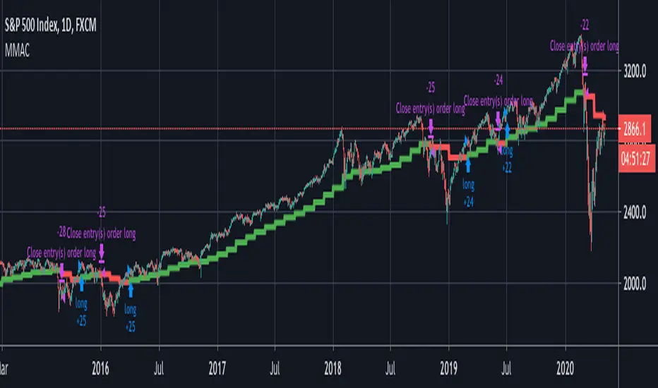
Average True Range Pivot(2) High and ATR tick colorsTakes original colored ATR tick code from Autarch_Capital and adds pivot (2) high. In image the green upticks are thickened to make them easier to see. Can change in settings.
Wyszukaj w skryptach "文华财经tick价格"
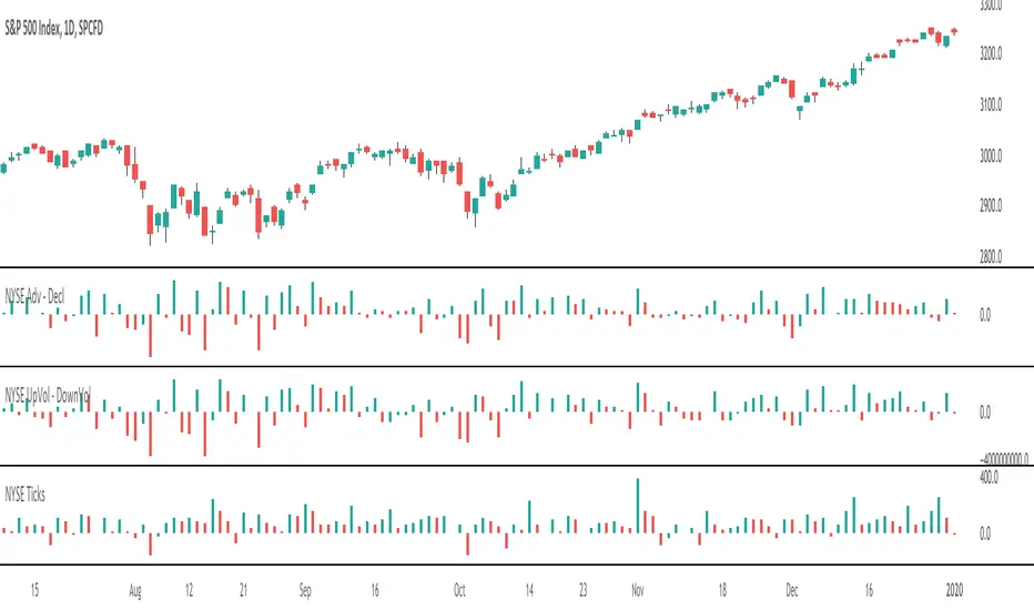
HG Scalpius - ATR Up/Down Tick HighlightHG Scalpius - ATR Up/Down Tick Highlight
This indicator highlights ATR(14) upticks (green) and downticks (red) and has the below application:
- If a new trend closing high (low) is made on a downtick in ATR, decreasing volatility mode turns on
If you come across or think of any other useful scripts for the HG Scalpius system please comment below!
Links to 2 previous HG Scalpius scripts:
-
-
Happy trading!
Code:
study(title="Average True Range", shorttitle="ATR", overlay=false)
length = input(title="Length", defval=14, minval=1)
smoothing = input(title="Smoothing", defval="RMA", options= )
ma_function(source, length) =>
if smoothing == "RMA"
rma(source, length)
else
if smoothing == "SMA"
sma(source, length)
else
if smoothing == "EMA"
ema(source, length)
else
wma(source, length)
ATR = ma_function(tr(true), length)
c = ATR >= ATR ? color.lime : color.red
plot(ATR, title = "ATR", color=c, transp=0)
Volume per minimum tickThis script calculates the volume traded per minimum tick of a scrip and is an indicator that the price move is justified by volume and trader interest
Strategy█ OVERVIEW
This library is a Pine Script™ programmer’s tool containing a variety of strategy-related functions to assist in calculations like profit and loss, stop losses and limits. It also includes several useful functions one can use to convert between units in ticks, price, currency or a percentage of the position's size.
█ CONCEPTS
The library contains three types of functions:
1 — Functions beginning with `percent` take either a portion of a price, or the current position's entry price and convert it to the value outlined in the function's documentation.
Example: Converting a percent of the current position entry price to ticks, or calculating a percent profit at a given level for the position.
2 — Functions beginning with `tick` convert a tick value to another form.
These are useful for calculating a price or currency value from a specified number of ticks.
3 — Functions containing `Level` are used to calculate a stop or take profit level using an offset in ticks from the current entry price.
These functions can be used to plot stop or take profit levels on the chart, or as arguments to the `limit` and `stop` parameters in strategy.exit() function calls.
Note that these calculated levels flip automatically with the position's bias.
For example, using `ticksToStopLevel()` will calculate a stop level under the entry price for a long position, and above the entry price for a short position.
There are also two functions to assist in calculating a position size using the entry's stop and a fixed risk expressed as a percentage of the current account's equity. By varying the position size this way, you ensure that entries with different stop levels risk the same proportion of equity.
█ NOTES
Example code using some of the library's functions is included at the end of the library. To see it in action, copy the library's code to a new script in the Pine Editor, and “Add to chart”.
For each trade, the code displays:
• The entry level in orange.
• The stop level in fuchsia.
• The take profit level in green.
The stop and take profit levels automatically flip sides based on whether the current position is long or short.
Labels near the last trade's levels display the percentages used to calculate them, which can be changed in the script's inputs.
We plot markers for entries and exits because strategy code in libraries does not display the usual markers for them.
Look first. Then leap.
█ FUNCTIONS
percentToTicks(percent) Converts a percentage of the average entry price to ticks.
Parameters:
percent : (series int/float) The percentage of `strategy.position_avg_price` to convert to ticks. 50 is 50% of the entry price.
Returns: (float) A value in ticks.
percentToPrice(percent) Converts a percentage of the average entry price to a price.
Parameters:
percent : (series int/float) The percentage of `strategy.position_avg_price` to convert to price. 50 is 50% of the entry price.
Returns: (float) A value in the symbol's quote currency (USD for BTCUSD).
percentToCurrency(price, percent) Converts the percentage of a price to money.
Parameters:
price : (series int/float) The symbol's price.
percent : (series int/float) The percentage of `price` to calculate.
Returns: (float) A value in the symbol's currency.
percentProfit(exitPrice) Calculates the profit (as a percentage of the position's `strategy.position_avg_price` entry price) if the trade is closed at `exitPrice`.
Parameters:
exitPrice : (series int/float) The potential price to close the position.
Returns: (float) Percentage profit for the current position if closed at the `exitPrice`.
priceToTicks(price) Converts a price to ticks.
Parameters:
price : (series int/float) Price to convert to ticks.
Returns: (float) A quantity of ticks.
ticksToPrice(price) Converts ticks to a price offset from the average entry price.
Parameters:
price : (series int/float) Ticks to convert to a price.
Returns: (float) A price level that has a distance from the entry price equal to the specified number of ticks.
ticksToCurrency(ticks) Converts ticks to money.
Parameters:
ticks : (series int/float) Number of ticks.
Returns: (float) Money amount in the symbol's currency.
ticksToStopLevel(ticks) Calculates a stop loss level using a distance in ticks from the current `strategy.position_avg_price` entry price. This value can be plotted on the chart, or used as an argument to the `stop` parameter of a `strategy.exit()` call. NOTE: The stop level automatically flips based on whether the position is long or short.
Parameters:
ticks : (series int/float) The distance in ticks from the entry price to the stop loss level.
Returns: (float) A stop loss level for the current position.
ticksToTpLevel(ticks) Calculates a take profit level using a distance in ticks from the current `strategy.position_avg_price` entry price. This value can be plotted on the chart, or used as an argument to the `limit` parameter of a `strategy.exit()` call. NOTE: The take profit level automatically flips based on whether the position is long or short.
Parameters:
ticks : (series int/float) The distance in ticks from the entry price to the take profit level.
Returns: (float) A take profit level for the current position.
calcPositionSizeByStopLossTicks(stopLossTicks, riskPercent) Calculates the position size needed to implement a given stop loss (in ticks) corresponding to `riskPercent` of equity.
Parameters:
stopLossTicks : (series int) The stop loss (in ticks) that will be used to protect the position.
riskPercent : (series int/float) The maximum risk level as a percent of current equity (`strategy.equity`).
Returns: (int) A quantity of contracts.
calcPositionSizeByStopLossPercent(stopLossPercent, riskPercent, entryPrice) Calculates the position size needed to implement a given stop loss (%) corresponding to `riskPercent` of equity.
Parameters:
stopLossPercent : (series int/float) The stop loss in percent that will be used to protect the position.
riskPercent : (series int/float) The maximum risk level as a percent of current equity (`strategy.equity`).
entryPrice : (series int/float) The entry price of the position.
Returns: (int) A quantity of contracts.
exitPercent(id, lossPercent, profitPercent, qty, qtyPercent, comment, when, alertMessage) A wrapper of the `strategy.exit()` built-in which adds the possibility to specify loss & profit in as a value in percent. NOTE: this function may work incorrectly with pyramiding turned on due to the use of `strategy.position_avg_price` in its calculations of stop loss and take profit offsets.
Parameters:
id : (series string) The order identifier of the `strategy.exit()` call.
lossPercent : (series int/float) Stop loss as a percent of the entry price.
profitPercent : (series int/float) Take profit as a percent of the entry price.
qty : (series int/float) Number of contracts/shares/lots/units to exit a trade with. The default value is `na`.
qtyPercent : (series int/float) The percent of the position's size to exit a trade with. If `qty` is `na`, the default value of `qty_percent` is 100.
comment : (series string) Optional. Additional notes on the order.
when : (series bool) Condition of the order. The order is placed if it is true.
alertMessage : (series string) An optional parameter which replaces the {{strategy.order.alert_message}} placeholder when it is used in the "Create Alert" dialog box's "Message" field.
ApicodeLibrary "Apicode"
percentToTicks(percent, from)
Converts a percentage of the average entry price or a specified price to ticks when the
strategy has an open position.
Parameters:
percent (float) : (series int/float) The percentage of the `from` price to express in ticks, e.g.,
a value of 50 represents 50% (half) of the price.
from (float) : (series int/float) Optional. The price from which to calculate a percentage and convert
to ticks. The default is `strategy.position_avg_price`.
Returns: (float) The number of ticks within the specified percentage of the `from` price if
the strategy has an open position. Otherwise, it returns `na`.
percentToPrice(percent, from)
Calculates the price value that is a specific percentage distance away from the average
entry price or a specified price when the strategy has an open position.
Parameters:
percent (float) : (series int/float) The percentage of the `from` price to use as the distance. If the value
is positive, the calculated price is above the `from` price. If negative, the result is
below the `from` price. For example, a value of 10 calculates the price 10% higher than
the `from` price.
from (float) : (series int/float) Optional. The price from which to calculate a percentage distance.
The default is `strategy.position_avg_price`.
Returns: (float) The price value at the specified `percentage` distance away from the `from` price
if the strategy has an open position. Otherwise, it returns `na`.
percentToCurrency(price, percent)
Parameters:
price (float) : (series int/float) The price from which to calculate the percentage.
percent (float) : (series int/float) The percentage of the `price` to calculate.
Returns: (float) The amount of the symbol's currency represented by the percentage of the specified
`price`.
percentProfit(exitPrice)
Calculates the expected profit/loss of the open position if it were to close at the
specified `exitPrice`, expressed as a percentage of the average entry price.
NOTE: This function may not return precise values for positions with multiple open trades
because it only uses the average entry price.
Parameters:
exitPrice (float) : (series int/float) The position's hypothetical closing price.
Returns: (float) The expected profit percentage from exiting the position at the `exitPrice`. If
there is no open position, it returns `na`.
priceToTicks(price)
Converts a price value to ticks.
Parameters:
price (float) : (series int/float) The price to convert.
Returns: (float) The value of the `price`, expressed in ticks.
ticksToPrice(ticks, from)
Calculates the price value at the specified number of ticks away from the average entry
price or a specified price when the strategy has an open position.
Parameters:
ticks (float) : (series int/float) The number of ticks away from the `from` price. If the value is positive,
the calculated price is above the `from` price. If negative, the result is below the `from`
price.
from (float) : (series int/float) Optional. The price to evaluate the tick distance from. The default is
`strategy.position_avg_price`.
Returns: (float) The price value at the specified number of ticks away from the `from` price if
the strategy has an open position. Otherwise, it returns `na`.
ticksToCurrency(ticks)
Converts a specified number of ticks to an amount of the symbol's currency.
Parameters:
ticks (float) : (series int/float) The number of ticks to convert.
Returns: (float) The amount of the symbol's currency represented by the tick distance.
ticksToStopLevel(ticks)
Calculates a stop-loss level using a specified tick distance from the position's average
entry price. A script can plot the returned value and use it as the `stop` argument in a
`strategy.exit()` call.
Parameters:
ticks (float) : (series int/float) The number of ticks from the position's average entry price to the
stop-loss level. If the position is long, the value represents the number of ticks *below*
the average entry price. If short, it represents the number of ticks *above* the price.
Returns: (float) The calculated stop-loss value for the open position. If there is no open position,
it returns `na`.
ticksToTpLevel(ticks)
Calculates a take-profit level using a specified tick distance from the position's average
entry price. A script can plot the returned value and use it as the `limit` argument in a
`strategy.exit()` call.
Parameters:
ticks (float) : (series int/float) The number of ticks from the position's average entry price to the
take-profit level. If the position is long, the value represents the number of ticks *above*
the average entry price. If short, it represents the number of ticks *below* the price.
Returns: (float) The calculated take-profit value for the open position. If there is no open
position, it returns `na`.
calcPositionSizeByStopLossTicks(stopLossTicks, riskPercent)
Calculates the entry quantity required to risk a specified percentage of the strategy's
current equity at a tick-based stop-loss level.
Parameters:
stopLossTicks (float) : (series int/float) The number of ticks in the stop-loss distance.
riskPercent (float) : (series int/float) The percentage of the strategy's equity to risk if a trade moves
`stopLossTicks` away from the entry price in the unfavorable direction.
Returns: (int) The number of contracts/shares/lots/units to use as the entry quantity to risk the
specified percentage of equity at the stop-loss level.
calcPositionSizeByStopLossPercent(stopLossPercent, riskPercent, entryPrice)
Calculates the entry quantity required to risk a specified percentage of the strategy's
current equity at a percent-based stop-loss level.
Parameters:
stopLossPercent (float) : (series int/float) The percentage of the `entryPrice` to use as the stop-loss distance.
riskPercent (float) : (series int/float) The percentage of the strategy's equity to risk if a trade moves
`stopLossPercent` of the `entryPrice` in the unfavorable direction.
entryPrice (float) : (series int/float) Optional. The entry price to use in the calculation. The default is
`close`.
Returns: (int) The number of contracts/shares/lots/units to use as the entry quantity to risk the
specified percentage of equity at the stop-loss level.
exitPercent(id, lossPercent, profitPercent, qty, qtyPercent, comment, alertMessage)
A wrapper for the `strategy.exit()` function designed for creating stop-loss and
take-profit orders at percentage distances away from the position's average entry price.
NOTE: This function calls `strategy.exit()` without a `from_entry` ID, so it creates exit
orders for *every* entry in an open position until the position closes. Therefore, using
this function when the strategy has a pyramiding value greater than 1 can lead to
unexpected results. See the "Exits for multiple entries" section of our User Manual's
"Strategies" page to learn more about this behavior.
Parameters:
id (string) : (series string) Optional. The identifier of the stop-loss/take-profit orders, which
corresponds to an exit ID in the strategy's trades after an order fills. The default is
`"Exit"`.
lossPercent (float) : (series int/float) The percentage of the position's average entry price to use as the
stop-loss distance. The function does not create a stop-loss order if the value is `na`.
profitPercent (float) : (series int/float) The percentage of the position's average entry price to use as the
take-profit distance. The function does not create a take-profit order if the value is `na`.
qty (float) : (series int/float) Optional. The number of contracts/lots/shares/units to close when an
exit order fills. If specified, the call uses this value instead of `qtyPercent` to
determine the order size. The exit orders reserve this quantity from the position, meaning
other orders from `strategy.exit()` cannot close this portion until the strategy fills or
cancels those orders. The default is `na`, which means the order size depends on the
`qtyPercent` value.
qtyPercent (float) : (series int/float) Optional. A value between 0 and 100 representing the percentage of the
open trade quantity to close when an exit order fills. The exit orders reserve this
percentage from the open trades, meaning other calls to this command cannot close this
portion until the strategy fills or cancels those orders. The percentage calculation
depends on the total size of the applicable open trades without considering the reserved
amount from other `strategy.exit()` calls. The call ignores this parameter if the `qty`
value is not `na`. The default is 100.
comment (string) : (series string) Optional. Additional notes on the filled order. If the value is specified
and not an empty "string", the Strategy Tester and the chart show this text for the order
instead of the specified `id`. The default is `na`.
alertMessage (string) : (series string) Optional. Custom text for the alert that fires when an order fills. If the
value is specified and not an empty "string", and the "Message" field of the "Create Alert"
dialog box contains the `{{strategy.order.alert_message}}` placeholder, the alert message
replaces the placeholder with this text. The default is `na`.
Returns: (void) The function does not return a usable value.
closeAllAtEndOfSession(comment, alertMessage)
A wrapper for the `strategy.close_all()` function designed to close all open trades with a
market order when the last bar in the current day's session closes. It uses the command's
`immediately` parameter to exit all trades at the last bar's `close` instead of the `open`
of the next session's first bar.
Parameters:
comment (string) : (series string) Optional. Additional notes on the filled order. If the value is specified
and not an empty "string", the Strategy Tester and the chart show this text for the order
instead of the automatically generated exit identifier. The default is `na`.
alertMessage (string) : (series string) Optional. Custom text for the alert that fires when an order fills. If the
value is specified and not an empty "string", and the "Message" field of the "Create Alert"
dialog box contains the `{{strategy.order.alert_message}}` placeholder, the alert message
replaces the placeholder with this text. The default is `na`.
Returns: (void) The function does not return a usable value.
closeAtEndOfSession(entryId, comment, alertMessage)
A wrapper for the `strategy.close()` function designed to close specific open trades with a
market order when the last bar in the current day's session closes. It uses the command's
`immediately` parameter to exit the trades at the last bar's `close` instead of the `open`
of the next session's first bar.
Parameters:
entryId (string)
comment (string) : (series string) Optional. Additional notes on the filled order. If the value is specified
and not an empty "string", the Strategy Tester and the chart show this text for the order
instead of the automatically generated exit identifier. The default is `na`.
alertMessage (string) : (series string) Optional. Custom text for the alert that fires when an order fills. If the
value is specified and not an empty "string", and the "Message" field of the "Create Alert"
dialog box contains the `{{strategy.order.alert_message}}` placeholder, the alert message
replaces the placeholder with this text. The default is `na`.
Returns: (void) The function does not return a usable value.
sortinoRatio(interestRate, forceCalc)
Calculates the Sortino ratio of the strategy based on realized monthly returns.
Parameters:
interestRate (simple float) : (simple int/float) Optional. The *annual* "risk-free" return percentage to compare against
strategy returns. The default is 2, meaning it uses an annual benchmark of 2%.
forceCalc (bool) : (series bool) Optional. A value of `true` forces the function to calculate the ratio on the
current bar. If the value is `false`, the function calculates the ratio only on the latest
available bar for efficiency. The default is `false`.
Returns: (float) The Sortino ratio, which estimates the strategy's excess return per unit of
downside volatility.
sharpeRatio(interestRate, forceCalc)
Calculates the Sharpe ratio of the strategy based on realized monthly returns.
Parameters:
interestRate (simple float) : (simple int/float) Optional. The *annual* "risk-free" return percentage to compare against
strategy returns. The default is 2, meaning it uses an annual benchmark of 2%.
forceCalc (bool) : (series bool) Optional. A value of `true` forces the function to calculate the ratio on the
current bar. If the value is `false`, the function calculates the ratio only on the latest
available bar for efficiency. The default is `false`.
Returns: (float) The Sortino ratio, which estimates the strategy's excess return per unit of
total volatility.
Waindrops [Makit0]█ OVERALL
Plot waindrops (custom volume profiles) on user defined periods, for each period you get high and low, it slices each period in half to get independent vwap, volume profile and the volume traded per price at each half.
It works on intraday charts only, up to 720m (12H). It can plot balanced or unbalanced waindrops, and volume profiles up to 24H sessions.
As example you can setup unbalanced periods to get independent volume profiles for the overnight and cash sessions on the futures market, or 24H periods to get the full session volume profile of EURUSD
The purpose of this indicator is twofold:
1 — from a Chartist point of view, to have an indicator which displays the volume in a more readable way
2 — from a Pine Coder point of view, to have an example of use for two very powerful tools on Pine Script:
• the recently updated drawing limit to 500 (from 50)
• the recently ability to use drawings arrays (lines and labels)
If you are new to Pine Script and you are learning how to code, I hope you read all the code and comments on this indicator, all is designed for you,
the variables and functions names, the sometimes too big explanations, the overall structure of the code, all is intended as an example on how to code
in Pine Script a specific indicator from a very good specification in form of white paper
If you wanna learn Pine Script form scratch just start HERE
In case you have any kind of problem with Pine Script please use some of the awesome resources at our disposal: USRMAN , REFMAN , AWESOMENESS , MAGIC
█ FEATURES
Waindrops are a different way of seeing the volume and price plotted in a chart, its a volume profile indicator where you can see the volume of each price level
plotted as a vertical histogram for each half of a custom period. By default the period is 60 so it plots an independent volume profile each 30m
You can think of each waindrop as an user defined candlestick or bar with four key values:
• high of the period
• low of the period
• left vwap (volume weighted average price of the first half period)
• right vwap (volume weighted average price of the second half period)
The waindrop can have 3 different colors (configurable by the user):
• GREEN: when the right vwap is higher than the left vwap (bullish sentiment )
• RED: when the right vwap is lower than the left vwap (bearish sentiment )
• BLUE: when the right vwap is equal than the left vwap ( neutral sentiment )
KEY FEATURES
• Help menu
• Custom periods
• Central bars
• Left/Right VWAPs
• Custom central bars and vwaps: color and pixels
• Highly configurable volume histogram: execution window, ticks, pixels, color, update frequency and fine tuning the neutral meaning
• Volume labels with custom size and color
• Tracking price dot to be able to see the current price when you hide your default candlesticks or bars
█ SETTINGS
Click here or set any impar period to see the HELP INFO : show the HELP INFO, if it is activated the indicator will not plot
PERIOD SIZE (max 2880 min) : waindrop size in minutes, default 60, max 2880 to allow the first half of a 48H period as a full session volume profile
BARS : show the central and vwap bars, default true
Central bars : show the central bars, default true
VWAP bars : show the left and right vwap bars, default true
Bars pixels : width of the bars in pixels, default 2
Bars color mode : bars color behavior
• BARS : gets the color from the 'Bars color' option on the settings panel
• HISTOGRAM : gets the color from the Bearish/Bullish/Neutral Histogram color options from the settings panel
Bars color : color for the central and vwap bars, default white
HISTOGRAM show the volume histogram, default true
Execution window (x24H) : last 24H periods where the volume funcionality will be plotted, default 5
Ticks per bar (max 50) : width in ticks of each histogram bar, default 2
Updates per period : number of times the histogram will update
• ONE : update at the last bar of the period
• TWO : update at the last bar of each half period
• FOUR : slice the period in 4 quarters and updates at the last bar of each of them
• EACH BAR : updates at the close of each bar
Pixels per bar : width in pixels of each histogram bar, default 4
Neutral Treshold (ticks) : delta in ticks between left and right vwaps to identify a waindrop as neutral, default 0
Bearish Histogram color : histogram color when right vwap is lower than left vwap, default red
Bullish Histogram color : histogram color when right vwap is higher than left vwap, default green
Neutral Histogram color : histogram color when the delta between right and left vwaps is equal or lower than the Neutral treshold, default blue
VOLUME LABELS : show volume labels
Volume labels color : color for the volume labels, default white
Volume Labels size : text size for the volume labels, choose between AUTO, TINY, SMALL, NORMAL or LARGE, default TINY
TRACK PRICE : show a yellow ball tracking the last price, default true
█ LIMITS
This indicator only works on intraday charts (minutes only) up to 12H (720m), the lower chart timeframe you can use is 1m
This indicator needs price, time and volume to work, it will not work on an index (there is no volume), the execution will not be allowed
The histogram (volume profile) can be plotted on 24H sessions as limit but you can plot several 24H sessions
█ ERRORS AND PERFORMANCE
Depending on the choosed settings, the script performance will be highly affected and it will experience errors
Two of the more common errors it can throw are:
• Calculation takes too long to execute
• Loop takes too long
The indicator performance is highly related to the underlying volatility (tick wise), the script takes each candlestick or bar and for each tick in it stores the price and volume, if the ticker in your chart has thousands and thousands of ticks per bar the indicator will throw an error for sure, it can not calculate in time such amount of ticks.
What all of that means? Simply put, this will throw error on the BITCOIN pair BTCUSD (high volatility with tick size 0.01) because it has too many ticks per bar, but lucky you it will work just fine on the futures contract BTC1! (tick size 5) because it has a lot less ticks per bar
There are some options you can fine tune to boost the script performance, the more demanding option in terms of resources consumption is Updates per period , by default is maxed out so lowering this setting will improve the performance in a high way.
If you wanna know more about how to improve the script performance, read the HELP INFO accessible from the settings panel
█ HOW-TO SETUP
The basic parameters to adjust are Period size , Ticks per bar and Pixels per bar
• Period size is the main setting, defines the waindrop size, to get a better looking histogram set bigger period and smaller chart timeframe
• Ticks per bar is the tricky one, adjust it differently for each underlying (ticker) volatility wise, for some you will need a low value, for others a high one.
To get a more accurate histogram set it as lower as you can (min value is 1)
• Pixels per bar allows you to adjust the width of each histogram bar, with it you can adjust the blank space between them or allow overlaping
You must play with these three parameters until you obtain the desired histogram: smoother, sharper, etc...
These are some of the different kind of charts you can setup thru the settings:
• Balanced Waindrops (default): charts with waindrops where the two halfs are of same size.
This is the default chart, just select a period (30m, 60m, 120m, 240m, pick your poison), adjust the histogram ticks and pixels and watch
• Unbalanced Waindrops: chart with waindrops where the two halfs are of different sizes.
Do you trade futures and want to plot a waindrop with the first half for the overnight session and the second half for the cash session? you got it;
just adjust the period to 1860 for any CME ticker (like ES1! for example) adjust the histogram ticks and pixels and watch
• Full Session Volume Profile: chart with waindrops where only the first half plots.
Do you use Volume profile to analize the market? Lucky you, now you can trick this one to plot it, just try a period of 780 on SPY, 2760 on ES1!, or 2880 on EURUSD
remember to adjust the histogram ticks and pixels for each underlying
• Only Bars: charts with only central and vwap bars plotted, simply deactivate the histogram and volume labels
• Only Histogram: charts with only the histogram plotted (volume profile charts), simply deactivate the bars and volume labels
• Only Volume: charts with only the raw volume numbers plotted, simply deactivate the bars and histogram
If you wanna know more about custom full session periods for different asset classes, read the HELP INFO accessible from the settings panel
EXAMPLES
Full Session Volume Profile on MES 5m chart:
Full Session Unbalanced Waindrop on MNQ 2m chart (left side Overnight session, right side Cash Session):
The following examples will have the exact same charts but on four different tickers representing a futures contract, a forex pair, an etf and a stock.
We are doing this to be able to see the different parameters we need for plotting the same kind of chart on different assets
The chart composition is as follows:
• Left side: Volume Labels chart (period 10)
• Upper Right side: Waindrops (period 60)
• Lower Right side: Full Session Volume Profile
The first example will specify the main parameters, the rest of the charts will have only the differences
MES :
• Left: Period size: 10, Bars: uncheck, Histogram: uncheck, Execution window: 1, Ticks per bar: 2, Updates per period: EACH BAR,
Pixels per bar: 4, Volume labels: check, Track price: check
• Upper Right: Period size: 60, Bars: check, Bars color mode: HISTOGRAM, Histogram: check, Execution window: 2, Ticks per bar: 2,
Updates per period: EACH BAR, Pixels per bar: 4, Volume labels: uncheck, Track price: check
• Lower Right: Period size: 2760, Bars: uncheck, Histogram: check, Execution window: 1, Ticks per bar: 1, Updates per period: EACH BAR,
Pixels per bar: 2, Volume labels: uncheck, Track price: check
EURUSD :
• Upper Right: Ticks per bar: 10
• Lower Right: Period size: 2880, Ticks per bar: 1, Pixels per bar: 1
SPY :
• Left: Ticks per bar: 3
• Upper Right: Ticks per bar: 5, Pixels per bar: 3
• Lower Right: Period size: 780, Ticks per bar: 2, Pixels per bar: 2
AAPL :
• Left: Ticks per bar: 2
• Upper Right: Ticks per bar: 6, Pixels per bar: 3
• Lower Right: Period size: 780, Ticks per bar: 1, Pixels per bar: 2
█ THANKS TO
PineCoders for all they do, all the tools and help they provide and their involvement in making a better community
scarf for the idea of coding a waindrops like indicator, I did not know something like that existed at all
All the Pine Coders, Pine Pros and Pine Wizards, people who share their work and knowledge for the sake of it and helping others, I'm very grateful indeed
I'm learning at each step of the way from you all, thanks for this awesome community;
Opensource and shared knowledge: this is the way! (said with canned voice from inside my helmet :D)
█ NOTE
This description was formatted following THIS guidelines
═════════════════════════════════════════════════════════════════════════
I sincerely hope you enjoy reading and using this work as much as I enjoyed developing it :D
GOOD LUCK AND HAPPY TRADING!
SMT Divergences [LuxAlgo]The SMT Divergences indicator highlights SMT divergences between the chart symbol and two user-selected tickers (ES and YM by default).
A dashboard returning the SMT divergences statistics is also provided within the settings.
🔶 SETTINGS
Swing Lookback: Calculation window used to detect swing points.
Comparison Ticker: If enabled, will detect SMT divergences between the chart prices and the prices of the selected ticker.
🔹 Dashboard
Show Dashboard: Displays statistics dashboard on the chart.
Location: Location of the dashboard on the chart.
Size: Size of the displayed dashboard.
🔶 USAGE
SMT Divergences are characterized by diverging swing points between two securities.
The detection of SMT Divergences is performed by detecting swing points using the user chart prices as well as the prices of the selected external tickers. If a swing point on the chart ticker is detected at the same time on external tickers, comparison is performed.
Due to the detection requiring swing point confirmation (3 candles by default), this indicator can better be used to study price behaviors on the occurrence of an SMT divergence.
The dashboard highlights the number of SMT divergences that occurred on a swing high and swing low between the chart ticker and the selected external tickers.
The returned percentage indicates the proportion of swing highs or swing lows that led to an SMT divergence.
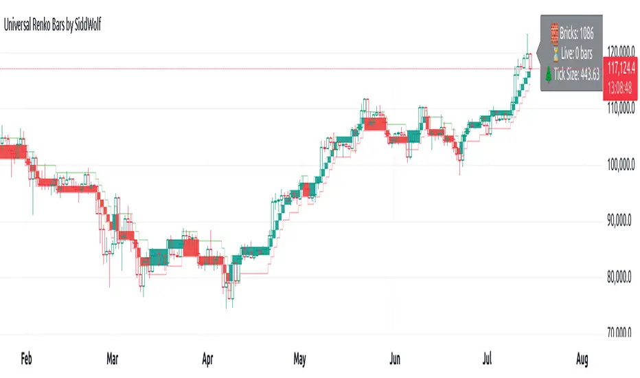
Universal Renko Bars by SiddWolfUniversal Renko Bars or UniRenko Bars is an overlay indicator that applies the logic of Renko charting directly onto a standard candlestick chart. It generates a sequence of price-driven bricks, where each new brick is formed only when the price moves a specific amount, regardless of time. This provides a clean, price-action-focused visualization of the market's trend.
WHAT IS UNIVERSAL RENKO BARS?
For years, traders have faced a stark choice: the clean, noise-free world of Renko charts, or the rich, time-based context of Candlesticks. Choosing Renko meant giving up your favorite moving averages, volume profiles, and the fundamental sense of time. Choosing Candlesticks meant enduring the market noise that often clouds true price action.
But what if you didn't have to choose?
Universal Renko Bars is a revolutionary indicator that ends this dilemma. It's not just another charting tool; it's a powerful synthesis that overlays the pure, price-driven logic of Renko bricks directly onto your standard candlestick chart. This hybrid approach gives you the best of both worlds:
❖ The Clarity of Renko: By filtering out the insignificant noise of time, Universal Renko reveals the underlying trend with unparalleled clarity. Up trends are clean successions of green bricks; down trends are clear red bricks. No more guesswork.
❖ The Context of Candlesticks: Because the Renko logic is an overlay, you retain your time axis, your volume data, and full compatibility with every other time-based indicator in your arsenal (RSI, MACD, Moving Averages, etc.).
The true magic, however, lies in its live, Unconfirmed Renko brick. This semi-transparent box is your window into the current bar's real-time struggle. It grows, shrinks, and changes color with every tick, showing you exactly how close the price is to confirming the trend or forcing a reversal. It’s no longer a lagging indicator; it’s a live look at the current battle between buyers and sellers.
Universal Renko Bars unifies these two powerful charting methods, transforming your chart into a more intelligent, noise-free, and predictive analytical canvas.
HOW TO USE
To get the most out of Universal Renko Bars, here are a few tips and a full breakdown of the settings.
Initial Setup for the Best Experience
For the cleanest possible view, it's highly recommended that you hide the body of your standard candlesticks, that shows only the skelton of the candle. This allows the Renko bricks to become the primary focus of your chart.
→ Double click on the candles and uncheck the body checkbox.
Settings Breakdown
The indicator is designed to be powerful yet intuitive. The settings are grouped to make customization easy.
First, What is a "Tick"?
Before we dive in, it's important to understand the concept of a "Tick." In Universal Renko, a Tick is not the same as a market tick. It's a fundamental unit of price movement that you define. For example, if you set the Tick Size to $0.50, then a price move of $1.00 is equal to 2 Ticks. This is the core building block for all Renko bricks. Tick size here is dynamically determined by the settings provided in the indicator.
❖ Calculation Method (The "Tick Size" Engine)
This section determines the monetary value of a single "Tick."
`Calculation Method` : Choose your preferred engine for defining the Tick Size.
`ATR Based` (Default): The Tick Size becomes dynamic, based on market volatility (Average True Range). Bricks will get larger in volatile markets and smaller in quiet ones. Use the `ATR 14 Multiplier` to control the sensitivity.
`Percentage` : The Tick Size is a simple percentage of the current asset price, controlled by the `Percent Size (%)` input.
`Auto` : The "set it and forget it" mode. The script intelligently calculates a Tick Size based on the asset's price. Use the `Auto Sensitivity` slider to make these automatically calculated bricks thicker (value > 1.0) or thinner (value < 1.0).
❖ Parameters (The Core Renko Engine)
This group controls how the bricks are constructed based on the Tick Size.
`Tick Trend` : The number of "Ticks" the price must move in the same direction to print a new continuation brick. A smaller value means bricks form more easily.
`Tick Reversal` : The number of "Ticks" the price must move in the opposite direction to print a new reversal brick. This is typically set higher than `Tick Trend` (e.g., double) to filter out minor pullbacks and market noise.
`Open Offset` : Controls the visual overlap of the bricks. A value of `0` creates gapless bricks that start where the last one ended. A value of `2` (with a `Tick Reversal` of 4) creates the classic 50% overlap look.
❖ Visuals (Controlling What You See)
This is where you tailor the chart to your visual preference.
`Show Confirmed Renko` : Toggles the solid-colored, historical bricks. These are finalized and will never change. They represent the confirmed past trend.
`Show Unconfirmed Renko` : This is the most powerful visual feature. It toggles the live, semi-transparent box that represents the developing brick. It shows you exactly where the price is right now in relation to the levels needed to form the next brick.
`Show Max/Min Levels` : Toggles the horizontal "finish lines" on your chart. The green line is the price target for a bullish brick, and the red line is the target for a bearish brick. These are excellent for spotting breakouts.
`Show Info Label` : Toggles the on-chart label that provides key real-time stats:
🧱 Bricks: The total count of confirmed bricks.
⏳ Live: How many chart bars the current live brick has been forming. These bars forms the Renko bricks that aren't confirmed yet. Live = 0 means the latest renko brick is confirmed.
🌲 Tick Size: The current calculated value of a single Tick.
Hover over the label for a tooltip with live RSI(14), MFI(14), and CCI(20) data for additional confirmation.
TRADING STRATEGIES & IDEAS
Universal Renko Bars isn't just a visual tool; it's a foundation for building robust trading strategies.
Trend Confirmation: The primary use is to instantly identify the trend. A series of green bricks indicates a strong uptrend; a series of red bricks indicates a strong downtrend. Use this to filter out trades that go against the primary momentum.
Reversal Spotting: Pay close attention to the Unconfirmed Brick . When a strong trend is in place and the live brick starts to fight against it—changing color and growing larger—it can be an early warning that a reversal is imminent. Wait for the brick to be confirmed for a higher probability entry.
Breakout Trading: The `Max/Min Levels` are your dynamic breakout zones. A long entry can be considered when the price breaks and closes above the green Max Level, confirming a new bullish brick. A short entry can be taken when price breaks below the red Min Level.
Confluence & Indicator Synergy: This is where Universal Renko truly shines. Overlay a moving average (e.g., 20 EMA). Only take long trades when the green bricks are forming above the EMA. Combine it with RSI or MACD; a bearish reversal brick forming while the RSI shows bearish divergence is a very powerful signal.
A FINAL WORD
Universal Renko Bars was designed to solve a fundamental problem in technical analysis. It brings together the best elements of two powerful methodologies to give you a clearer, more actionable view of the market. By filtering noise while retaining context, it empowers you to make decisions with greater confidence.
Add Universal Renko Bars to your chart today and elevate your analysis. We welcome your feedback and suggestions for future updates!
Follow me to get notified when I publish New Indicator.
~ SiddWolf
Yelober_Momentum_BreadthMI# Yelober_Momentum_BreadthMI: Market Breadth Indicator Analysis
## Overview
The Yelober_Momentum_BreadthMI is a comprehensive market breadth indicator designed to monitor market internals across NYSE and NASDAQ exchanges. It tracks several key metrics including up/down volume ratios, TICK readings, and trend momentum to provide traders with real-time insights into market direction, strength, and potential turning points.
## Indicator Components
This indicator displays a table with data for:
- NYSE breadth metrics
- NASDAQ breadth metrics
- NYSE TICK data and trends
- NASDAQ TICK (TICKQ) data and trends
## Table Columns and Interpretation
### Column 1: Market
Identifies the data source:
- **NYSE**: New York Stock Exchange data
- **NASDAQ**: NASDAQ exchange data
- **Tick**: NYSE TICK index
- **TickQ**: NASDAQ TICK index
### Column 2: Ratio
Shows the current ratio values with different calculations depending on the row:
- **For NYSE/NASDAQ rows**: Displays the up/down volume ratio
- Positive values (green): More up volume than down volume
- Negative values (red): More down volume than up volume
- The magnitude indicates the strength of the imbalance
- **For Tick/TickQ rows**: Shows the ratio of positive to negative ticks plus the current TICK reading in parentheses
- Format: "Ratio (Current TICK value)"
- Positive values (green): More stocks ticking up than down
- Negative values (red): More stocks ticking down than up
### Column 3: Trend
Displays the directional trend with both a symbol and value:
- **For NYSE/NASDAQ rows**: Shows the VOLD (volume difference) slope
- "↗": Rising trend (positive slope)
- "↘": Falling trend (negative slope)
- "→": Neutral/flat trend (minimal slope)
- **For Tick/TickQ rows**: Shows the slope of the ratio history
- Color-coding: Green for positive momentum, Red for negative momentum, Gray for neutral
The trend column is particularly important as it shows the current momentum of the market. The indicator applies specific thresholds for color-coding:
- NYSE: Green when normalized value > 2, Red when < -2
- NASDAQ: Green when normalized value > 3.5, Red when < -3.5
- TICK/TICKQ: Green when slope > 0.01, Red when slope < -0.01
## How to Use This Indicator
### Basic Interpretation
1. **Market Direction**: When multiple rows show green ratios and upward trends, it suggests strong bullish market internals. Conversely, red ratios and downward trends indicate bearish internals.
2. **Market Breadth**: The magnitude of the ratios indicates how broad-based the market movement is. Higher absolute values suggest stronger market breadth.
3. **Momentum Shifts**: When trend arrows change direction or colors shift, it may signal a potential reversal or change in market momentum.
4. **Divergences**: Look for divergences between different markets (NYSE vs NASDAQ) or between ratios and trends, which can indicate potential market turning points.
### Advanced Usage
- **Volume Normalization**: The indicator includes options to normalize volume data (none, tens, thousands, millions, 10th millions) to handle different exchange scales.
- **Trend Averaging**: The slope calculation uses an averaging period (default: 5) to smooth out noise and identify more reliable trend signals.
## Examples for Interpretation
### Example 1: Strong Bullish Market
```
| Market | Ratio | Trend |
|--------|---------|-----------|
| NYSE | 1.75 | ↗ 2.85 |
| NASDAQ | 2.10 | ↗ 4.12 |
| Tick | 2.45 (485) | ↗ 0.05 |
| TickQ | 1.95 (320) | ↗ 0.03 |
```
**Interpretation**: All metrics are positive and trending upward (green), indicating a strong, broad-based rally. The high ratio values show significant bullish dominance. This suggests continuation of the upward move with good momentum.
### Example 2: Weakening Market
```
| Market | Ratio | Trend |
|--------|---------|-----------|
| NYSE | 0.45 | ↘ -1.50 |
| NASDAQ | 0.85 | → 0.30 |
| Tick | 0.95 (105) | ↘ -0.02 |
| TickQ | 1.20 (160) | → 0.00 |
```
**Interpretation**: The market is showing mixed signals with positive but low ratios, while NYSE and TICK trends are turning negative. NASDAQ shows neutral to slightly positive momentum. This divergence often occurs near market tops or during consolidation phases. Traders should be cautious and consider reducing position sizes.
### Example 3: Negative Market Turning Positive
```
| Market | Ratio | Trend |
|--------|---------|-----------|
| NYSE | -1.25 | ↗ 1.75 |
| NASDAQ | -0.95 | ↗ 2.80 |
| Tick | -1.35 (-250) | ↗ 0.04 |
| TickQ | -1.10 (-180) | ↗ 0.02 |
```
**Interpretation**: This is a potential bottoming pattern. Current ratios are still negative (red) showing overall negative breadth, but the trends are all positive (green arrows), indicating improving momentum. This divergence often occurs at market bottoms and could signal an upcoming reversal. Look for confirmation with price action before establishing long positions.
### Example 4: Mixed Market with Divergence
```
| Market | Ratio | Trend |
|--------|---------|-----------|
| NYSE | 1.45 | ↘ -2.25 |
| NASDAQ | -0.85 | ↘ -3.80 |
| Tick | 1.20 (230) | ↘ -0.03 |
| TickQ | -0.75 (-120) | ↘ -0.02 |
```
**Interpretation**: There's a significant divergence between NYSE (positive ratio) and NASDAQ (negative ratio), while all trends are negative. This suggests sector rotation or a market that's weakening but with certain segments still showing strength. Often seen during late-stage bull markets or in transitions between leadership groups. Consider reducing risk exposure and focusing on relative strength sectors.
## Practical Trading Applications
1. **Confirmation Tool**: Use this indicator to confirm price movements. Strong breadth readings in the direction of the price trend increase confidence in trade decisions.
2. **Early Warning System**: Watch for divergences between price and breadth metrics, which often precede market turns.
3. **Intraday Trading**: The real-time nature of TICK and volume data makes this indicator valuable for day traders to gauge intraday momentum shifts.
4. **Market Regime Identification**: Sustained readings can help identify whether the market is in a trend or chop regime, allowing for appropriate strategy selection.
This breadth indicator is most effective when used in conjunction with price action and other technical indicators rather than in isolation.
Correlation Clusters [LuxAlgo]The Correlation Clusters is a machine learning tool that allows traders to group sets of tickers with a similar correlation coefficient to a user-set reference ticker.
The tool calculates the correlation coefficients between 10 user-set tickers and a user-set reference ticker, with the possibility of forming up to 10 clusters.
🔶 USAGE
Applying clustering methods to correlation analysis allows traders to quickly identify which set of tickers are correlated with a reference ticker, rather than having to look at them one by one or using a more tedious approach such as correlation matrices.
Tickers belonging to a cluster may also be more likely to have a higher mutual correlation. The image above shows the detailed parts of the Correlation Clusters tool.
The correlation coefficient between two assets allows traders to see how these assets behave in relation to each other. It can take values between +1.0 and -1.0 with the following meaning
Value near +1.0: Both assets behave in a similar way, moving up or down at the same time
Value close to 0.0: No correlation, both assets behave independently
Value near -1.0: Both assets have opposite behavior when one moves up the other moves down, and vice versa
There is a wide range of trading strategies that make use of correlation coefficients between assets, some examples are:
Pair Trading: Traders may wish to take advantage of divergences in the price movements of highly positively correlated assets; even highly positively correlated assets do not always move in the same direction; when assets with a correlation close to +1.0 diverge in their behavior, traders may see this as an opportunity to buy one and sell the other in the expectation that the assets will return to the likely same price behavior.
Sector rotation: Traders may want to favor some sectors that are expected to perform in the next cycle, tracking the correlation between different sectors and between the sector and the overall market.
Diversification: Traders can aim to have a diversified portfolio of uncorrelated assets. From a risk management perspective, it is useful to know the correlation between the assets in your portfolio, if you hold equal positions in positively correlated assets, your risk is tilted in the same direction, so if the assets move against you, your risk is doubled. You can avoid this increased risk by choosing uncorrelated assets so that they move independently.
Hedging: Traders may want to hedge positions with correlated assets, from a hedging perspective, if you are long an asset, you can hedge going long a negatively correlated asset or going short a positively correlated asset.
Grouping different assets with similar behavior can be very helpful to traders to avoid over-exposure to those assets, traders may have multiple long positions on different assets as a way of minimizing overall risk when in reality if those assets are part of the same cluster traders are maximizing their risk by taking positions on assets with the same behavior.
As a rule of thumb, a trader can minimize risk via diversification by taking positions on assets with no correlations, the proposed tool can effectively show a set of uncorrelated candidates from the reference ticker if one or more clusters centroids are located near 0.
🔶 DETAILS
K-means clustering is a popular machine-learning algorithm that finds observations in a data set that are similar to each other and places them in a group.
The process starts by randomly assigning each data point to an initial group and calculating the centroid for each. A centroid is the center of the group. K-means clustering forms the groups in such a way that the variances between the data points and the centroid of the cluster are minimized.
It's an unsupervised method because it starts without labels and then forms and labels groups itself.
🔹 Execution Window
In the image above we can see how different execution windows provide different correlation coefficients, informing traders of the different behavior of the same assets over different time periods.
Users can filter the data used to calculate correlations by number of bars, by time, or not at all, using all available data. For example, if the chart timeframe is 15m, traders may want to know how different assets behave over the last 7 days (one week), or for an hourly chart set an execution window of one month, or one year for a daily chart. The default setting is to use data from the last 50 bars.
🔹 Clusters
On this graph, we can see different clusters for the same data. The clusters are identified by different colors and the dotted lines show the centroids of each cluster.
Traders can select up to 10 clusters, however, do note that selecting 10 clusters can lead to only 4 or 5 returned clusters, this is caused by the machine learning algorithm not detecting any more data points deviating from already detected clusters.
Traders can fine-tune the algorithm by changing the 'Cluster Threshold' and 'Max Iterations' settings, but if you are not familiar with them we advise you not to change these settings, the defaults can work fine for the application of this tool.
🔹 Correlations
Different correlations mean different behaviors respecting the same asset, as we can see in the chart above.
All correlations are found against the same asset, traders can use the chart ticker or manually set one of their choices from the settings panel. Then they can select the 10 tickers to be used to find the correlation coefficients, which can be useful to analyze how different types of assets behave against the same asset.
🔶 SETTINGS
Execution Window Mode: Choose how the tool collects data, filter data by number of bars, time, or no filtering at all, using all available data.
Execute on Last X Bars: Number of bars for data collection when the 'Bars' execution window mode is active.
Execute on Last: Time window for data collection when the `Time` execution window mode is active. These are full periods, so `Day` means the last 24 hours, `Week` means the last 7 days, and so on.
🔹 Clusters
Number of Clusters: Number of clusters to detect up to 10. Only clusters with data points are displayed.
Cluster Threshold: Number used to compare a new centroid within the same cluster. The lower the number, the more accurate the centroid will be.
Max Iterations: Maximum number of calculations to detect a cluster. A high value may lead to a timeout runtime error (loop takes too long).
🔹 Ticker of Reference
Use Chart Ticker as Reference: Enable/disable the use of the current chart ticker to get the correlation against all other tickers selected by the user.
Custom Ticker: Custom ticker to get the correlation against all the other tickers selected by the user.
🔹 Correlation Tickers
Select the 10 tickers for which you wish to obtain the correlation against the reference ticker.
🔹 Style
Text Size: Select the size of the text to be displayed.
Display Size: Select the size of the correlation chart to be displayed, up to 500 bars.
Box Height: Select the height of the boxes to be displayed. A high height will cause overlapping if the boxes are close together.
Clusters Colors: Choose a custom colour for each cluster.
TRADINGLibrary "TRADING"
This library is a client script for making a webhook signal formatted string to PoABOT server.
entry_message(password, percent, leverage, margin_mode, kis_number)
Create a entry message for POABOT
Parameters:
password (string) : (string) The password of your bot.
percent (float) : (float) The percent for entry based on your wallet balance.
leverage (int) : (int) The leverage of entry. If not set, your levereage doesn't change.
margin_mode (string) : (string) The margin mode for trade(only for OKX). "cross" or "isolated"
kis_number (int) : (int) The number of koreainvestment account. Default 1
Returns: (string) A json formatted string for webhook message.
order_message(password, percent, leverage, margin_mode, kis_number)
Create a order message for POABOT
Parameters:
password (string) : (string) The password of your bot.
percent (float) : (float) The percent for entry based on your wallet balance.
leverage (int) : (int) The leverage of entry. If not set, your levereage doesn't change.
margin_mode (string) : (string) The margin mode for trade(only for OKX). "cross" or "isolated"
kis_number (int) : (int) The number of koreainvestment account. Default 1
Returns: (string) A json formatted string for webhook message.
close_message(password, percent, margin_mode, kis_number)
Create a close message for POABOT
Parameters:
password (string) : (string) The password of your bot.
percent (float) : (float) The percent for close based on your wallet balance.
margin_mode (string) : (string) The margin mode for trade(only for OKX). "cross" or "isolated"
kis_number (int) : (int) The number of koreainvestment account. Default 1
Returns: (string) A json formatted string for webhook message.
exit_message(password, percent, margin_mode, kis_number)
Create a exit message for POABOT
Parameters:
password (string) : (string) The password of your bot.
percent (float) : (float) The percent for exit based on your wallet balance.
margin_mode (string) : (string) The margin mode for trade(only for OKX). "cross" or "isolated"
kis_number (int) : (int) The number of koreainvestment account. Default 1
Returns: (string) A json formatted string for webhook message.
manual_message(password, exchange, base, quote, side, qty, price, percent, leverage, margin_mode, kis_number, order_name)
Create a manual message for POABOT
Parameters:
password (string) : (string) The password of your bot.
exchange (string) : (string) The exchange
base (string) : (string) The base
quote (string) : (string) The quote of order message
side (string) : (string) The side of order messsage
qty (float) : (float) The qty of order message
price (float) : (float) The price of order message
percent (float) : (float) The percent for order based on your wallet balance.
leverage (int) : (int) The leverage of entry. If not set, your levereage doesn't change.
margin_mode (string) : (string) The margin mode for trade(only for OKX). "cross" or "isolated"
kis_number (int) : (int) The number of koreainvestment account.
order_name (string) : (string) The name of order message
Returns: (string) A json formatted string for webhook message.
in_trade(start_time, end_time, hide_trade_line)
Create a trade start line
Parameters:
start_time (int) : (int) The start of time.
end_time (int) : (int) The end of time.
hide_trade_line (bool) : (bool) if true, hide trade line. Default false.
Returns: (bool) Get bool for trade based on time range.
real_qty(qty, precision, leverage, contract_size, default_qty_type, default_qty_value)
Get exchange specific real qty
Parameters:
qty (float) : (float) qty
precision (float) : (float) precision
leverage (int) : (int) leverage
contract_size (float) : (float) contract_size
default_qty_type (string)
default_qty_value (float)
Returns: (float) exchange specific qty.
method set(this, password, start_time, end_time, leverage, initial_capital, default_qty_type, default_qty_value, margin_mode, contract_size, kis_number, entry_percent, close_percent, exit_percent, fixed_qty, fixed_cash, real, auto_alert_message, hide_trade_line)
Set bot object.
Namespace types: bot
Parameters:
this (bot)
password (string) : (string) password for poabot.
start_time (int) : (int) start_time timestamp.
end_time (int) : (int) end_time timestamp.
leverage (int) : (int) leverage.
initial_capital (float)
default_qty_type (string)
default_qty_value (float)
margin_mode (string) : (string) The margin mode for trade(only for OKX). "cross" or "isolated"
contract_size (float)
kis_number (int) : (int) kis_number for poabot.
entry_percent (float) : (float) entry_percent for poabot.
close_percent (float) : (float) close_percent for poabot.
exit_percent (float) : (float) exit_percent for poabot.
fixed_qty (float) : (float) fixed qty.
fixed_cash (float) : (float) fixed cash.
real (bool) : (bool) convert qty for exchange specific.
auto_alert_message (bool) : (bool) convert alert_message for exchange specific.
hide_trade_line (bool) : (bool) if true, Hide trade line. Default false.
Returns: (void)
method print(this, message)
Print message using log table.
Namespace types: bot
Parameters:
this (bot)
message (string)
Returns: (void)
method start_trade(this)
start trade using start_time and end_time
Namespace types: bot
Parameters:
this (bot)
Returns: (void)
method entry(this, id, direction, qty, limit, stop, oca_name, oca_type, comment, alert_message, when)
It is a command to enter market position. If an order with the same ID is already pending, it is possible to modify the order. If there is no order with the specified ID, a new order is placed. To deactivate an entry order, the command strategy.cancel or strategy.cancel_all should be used. In comparison to the function strategy.order, the function strategy.entry is affected by pyramiding and it can reverse market position correctly. If both 'limit' and 'stop' parameters are 'NaN', the order type is market order.
Namespace types: bot
Parameters:
this (bot)
id (string) : (string) A required parameter. The order identifier. It is possible to cancel or modify an order by referencing its identifier.
direction (string) : (string) A required parameter. Market position direction: 'strategy.long' is for long, 'strategy.short' is for short.
qty (float) : (float) An optional parameter. Number of contracts/shares/lots/units to trade. The default value is 'NaN'.
limit (float) : (float) An optional parameter. Limit price of the order. If it is specified, the order type is either 'limit', or 'stop-limit'. 'NaN' should be specified for any other order type.
stop (float) : (float) An optional parameter. Stop price of the order. If it is specified, the order type is either 'stop', or 'stop-limit'. 'NaN' should be specified for any other order type.
oca_name (string) : (string) An optional parameter. Name of the OCA group the order belongs to. If the order should not belong to any particular OCA group, there should be an empty string.
oca_type (string) : (string) An optional parameter. Type of the OCA group. The allowed values are: "strategy.oca.none" - the order should not belong to any particular OCA group; "strategy.oca.cancel" - the order should belong to an OCA group, where as soon as an order is filled, all other orders of the same group are cancelled; "strategy.oca.reduce" - the order should belong to an OCA group, where if X number of contracts of an order is filled, number of contracts for each other order of the same OCA group is decreased by X.
comment (string) : (string) An optional parameter. Additional notes on the order.
alert_message (string) : (string) An optional parameter which replaces the {{strategy.order.alert_message}} placeholder when it is used in the "Create Alert" dialog box's "Message" field.
when (bool) : (bool) An optional parmeter. Condition, deprecated.
Returns: (void)
method order(this, id, direction, qty, limit, stop, oca_name, oca_type, comment, alert_message, when)
It is a command to place order. If an order with the same ID is already pending, it is possible to modify the order. If there is no order with the specified ID, a new order is placed. To deactivate order, the command strategy.cancel or strategy.cancel_all should be used. In comparison to the function strategy.entry, the function strategy.order is not affected by pyramiding. If both 'limit' and 'stop' parameters are 'NaN', the order type is market order.
Namespace types: bot
Parameters:
this (bot)
id (string) : (string) A required parameter. The order identifier. It is possible to cancel or modify an order by referencing its identifier.
direction (string) : (string) A required parameter. Market position direction: 'strategy.long' is for long, 'strategy.short' is for short.
qty (float) : (float) An optional parameter. Number of contracts/shares/lots/units to trade. The default value is 'NaN'.
limit (float) : (float) An optional parameter. Limit price of the order. If it is specified, the order type is either 'limit', or 'stop-limit'. 'NaN' should be specified for any other order type.
stop (float) : (float) An optional parameter. Stop price of the order. If it is specified, the order type is either 'stop', or 'stop-limit'. 'NaN' should be specified for any other order type.
oca_name (string) : (string) An optional parameter. Name of the OCA group the order belongs to. If the order should not belong to any particular OCA group, there should be an empty string.
oca_type (string) : (string) An optional parameter. Type of the OCA group. The allowed values are: "strategy.oca.none" - the order should not belong to any particular OCA group; "strategy.oca.cancel" - the order should belong to an OCA group, where as soon as an order is filled, all other orders of the same group are cancelled; "strategy.oca.reduce" - the order should belong to an OCA group, where if X number of contracts of an order is filled, number of contracts for each other order of the same OCA group is decreased by X.
comment (string) : (string) An optional parameter. Additional notes on the order.
alert_message (string) : (string) An optional parameter which replaces the {{strategy.order.alert_message}} placeholder when it is used in the "Create Alert" dialog box's "Message" field.
when (bool) : (bool) An optional parmeter. Condition, deprecated.
Returns: (void)
method close_all(this, comment, alert_message, immediately, when)
Exits the current market position, making it flat.
Namespace types: bot
Parameters:
this (bot)
comment (string) : (string) An optional parameter. Additional notes on the order.
alert_message (string) : (string) An optional parameter which replaces the {{strategy.order.alert_message}} placeholder when it is used in the "Create Alert" dialog box's "Message" field.
immediately (bool) : (bool) An optional parameter. If true, the closing order will be executed on the tick where it has been placed, ignoring the strategy parameters that restrict the order execution to the open of the next bar. The default is false.
when (bool) : (bool) An optional parmeter. Condition, deprecated.
Returns: (void)
method cancel(this, id, when)
It is a command to cancel/deactivate pending orders by referencing their names, which were generated by the functions: strategy.order, strategy.entry and strategy.exit.
Namespace types: bot
Parameters:
this (bot)
id (string) : (string) A required parameter. The order identifier. It is possible to cancel an order by referencing its identifier.
when (bool) : (bool) An optional parmeter. Condition, deprecated.
Returns: (void)
method cancel_all(this, when)
It is a command to cancel/deactivate all pending orders, which were generated by the functions: strategy.order, strategy.entry and strategy.exit.
Namespace types: bot
Parameters:
this (bot)
when (bool) : (bool) An optional parmeter. Condition, deprecated.
Returns: (void)
method close(this, id, comment, qty, qty_percent, alert_message, immediately, when)
It is a command to exit from the entry with the specified ID. If there were multiple entry orders with the same ID, all of them are exited at once. If there are no open entries with the specified ID by the moment the command is triggered, the command will not come into effect. The command uses market order. Every entry is closed by a separate market order.
Namespace types: bot
Parameters:
this (bot)
id (string) : (string) A required parameter. The order identifier. It is possible to close an order by referencing its identifier.
comment (string) : (string) An optional parameter. Additional notes on the order.
qty (float) : (float) An optional parameter. Number of contracts/shares/lots/units to exit a trade with. The default value is 'NaN'.
qty_percent (float) : (float) Defines the percentage (0-100) of the position to close. Its priority is lower than that of the 'qty' parameter. Optional. The default is 100.
alert_message (string) : (string) An optional parameter which replaces the {{strategy.order.alert_message}} placeholder when it is used in the "Create Alert" dialog box's "Message" field.
immediately (bool) : (bool) An optional parameter. If true, the closing order will be executed on the tick where it has been placed, ignoring the strategy parameters that restrict the order execution to the open of the next bar. The default is false.
when (bool) : (bool) An optional parmeter. Condition, deprecated.
Returns: (void)
ticks_to_price(ticks, from)
Converts ticks to a price offset from the supplied price or the average entry price.
Parameters:
ticks (float) : (float) Ticks to convert to a price.
from (float) : (float) A price that can be used to calculate from. Optional. The default value is `strategy.position_avg_price`.
Returns: (float) A price level that has a distance from the entry price equal to the specified number of ticks.
method exit(this, id, from_entry, qty, qty_percent, profit, limit, loss, stop, trail_price, trail_points, trail_offset, oca_name, comment, comment_profit, comment_loss, comment_trailing, alert_message, alert_profit, alert_loss, alert_trailing, when)
It is a command to exit either a specific entry, or whole market position. If an order with the same ID is already pending, it is possible to modify the order. If an entry order was not filled, but an exit order is generated, the exit order will wait till entry order is filled and then the exit order is placed. To deactivate an exit order, the command strategy.cancel or strategy.cancel_all should be used. If the function strategy.exit is called once, it exits a position only once. If you want to exit multiple times, the command strategy.exit should be called multiple times. If you use a stop loss and a trailing stop, their order type is 'stop', so only one of them is placed (the one that is supposed to be filled first). If all the following parameters 'profit', 'limit', 'loss', 'stop', 'trail_points', 'trail_offset' are 'NaN', the command will fail. To use market order to exit, the command strategy.close or strategy.close_all should be used.
Namespace types: bot
Parameters:
this (bot)
id (string) : (string) A required parameter. The order identifier. It is possible to cancel or modify an order by referencing its identifier.
from_entry (string) : (string) An optional parameter. The identifier of a specific entry order to exit from it. To exit all entries an empty string should be used. The default values is empty string.
qty (float) : (float) An optional parameter. Number of contracts/shares/lots/units to exit a trade with. The default value is 'NaN'.
qty_percent (float) : (float) Defines the percentage of (0-100) the position to close. Its priority is lower than that of the 'qty' parameter. Optional. The default is 100.
profit (float) : (float) An optional parameter. Profit target (specified in ticks). If it is specified, a limit order is placed to exit market position when the specified amount of profit (in ticks) is reached. The default value is 'NaN'.
limit (float) : (float) An optional parameter. Profit target (requires a specific price). If it is specified, a limit order is placed to exit market position at the specified price (or better). Priority of the parameter 'limit' is higher than priority of the parameter 'profit' ('limit' is used instead of 'profit', if its value is not 'NaN'). The default value is 'NaN'.
loss (float) : (float) An optional parameter. Stop loss (specified in ticks). If it is specified, a stop order is placed to exit market position when the specified amount of loss (in ticks) is reached. The default value is 'NaN'.
stop (float) : (float) An optional parameter. Stop loss (requires a specific price). If it is specified, a stop order is placed to exit market position at the specified price (or worse). Priority of the parameter 'stop' is higher than priority of the parameter 'loss' ('stop' is used instead of 'loss', if its value is not 'NaN'). The default value is 'NaN'.
trail_price (float) : (float) An optional parameter. Trailing stop activation level (requires a specific price). If it is specified, a trailing stop order will be placed when the specified price level is reached. The offset (in ticks) to determine initial price of the trailing stop order is specified in the 'trail_offset' parameter: X ticks lower than activation level to exit long position; X ticks higher than activation level to exit short position. The default value is 'NaN'.
trail_points (float) : (float) An optional parameter. Trailing stop activation level (profit specified in ticks). If it is specified, a trailing stop order will be placed when the calculated price level (specified amount of profit) is reached. The offset (in ticks) to determine initial price of the trailing stop order is specified in the 'trail_offset' parameter: X ticks lower than activation level to exit long position; X ticks higher than activation level to exit short position. The default value is 'NaN'.
trail_offset (float) : (float) An optional parameter. Trailing stop price (specified in ticks). The offset in ticks to determine initial price of the trailing stop order: X ticks lower than 'trail_price' or 'trail_points' to exit long position; X ticks higher than 'trail_price' or 'trail_points' to exit short position. The default value is 'NaN'.
oca_name (string) : (string) An optional parameter. Name of the OCA group (oca_type = strategy.oca.reduce) the profit target, the stop loss / the trailing stop orders belong to. If the name is not specified, it will be generated automatically.
comment (string) : (string) Additional notes on the order. If specified, displays near the order marker on the chart. Optional. The default is na.
comment_profit (string) : (string) Additional notes on the order if the exit was triggered by crossing `profit` or `limit` specifically. If specified, supercedes the `comment` parameter and displays near the order marker on the chart. Optional. The default is na.
comment_loss (string) : (string) Additional notes on the order if the exit was triggered by crossing `stop` or `loss` specifically. If specified, supercedes the `comment` parameter and displays near the order marker on the chart. Optional. The default is na.
comment_trailing (string) : (string) Additional notes on the order if the exit was triggered by crossing `trail_offset` specifically. If specified, supercedes the `comment` parameter and displays near the order marker on the chart. Optional. The default is na.
alert_message (string) : (string) Text that will replace the '{{strategy.order.alert_message}}' placeholder when one is used in the "Message" field of the "Create Alert" dialog. Optional. The default is na.
alert_profit (string) : (string) Text that will replace the '{{strategy.order.alert_message}}' placeholder when one is used in the "Message" field of the "Create Alert" dialog. Only replaces the text if the exit was triggered by crossing `profit` or `limit` specifically. Optional. The default is na.
alert_loss (string) : (string) Text that will replace the '{{strategy.order.alert_message}}' placeholder when one is used in the "Message" field of the "Create Alert" dialog. Only replaces the text if the exit was triggered by crossing `stop` or `loss` specifically. Optional. The default is na.
alert_trailing (string) : (string) Text that will replace the '{{strategy.order.alert_message}}' placeholder when one is used in the "Message" field of the "Create Alert" dialog. Only replaces the text if the exit was triggered by crossing `trail_offset` specifically. Optional. The default is na.
when (bool) : (bool) An optional parmeter. Condition, deprecated.
Returns: (void)
percent_to_ticks(percent, from)
Converts a percentage of the supplied price or the average entry price to ticks.
Parameters:
percent (float) : (float) The percentage of supplied price to convert to ticks. 50 is 50% of the entry price.
from (float) : (float) A price that can be used to calculate from. Optional. The default value is `strategy.position_avg_price`.
Returns: (float) A value in ticks.
percent_to_price(percent, from)
Converts a percentage of the supplied price or the average entry price to a price.
Parameters:
percent (float) : (float) The percentage of the supplied price to convert to price. 50 is 50% of the supplied price.
from (float) : (float) A price that can be used to calculate from. Optional. The default value is `strategy.position_avg_price`.
Returns: (float) A value in the symbol's quote currency (USD for BTCUSD).
bot
Fields:
password (series__string)
start_time (series__integer)
end_time (series__integer)
leverage (series__integer)
initial_capital (series__float)
default_qty_type (series__string)
default_qty_value (series__float)
margin_mode (series__string)
contract_size (series__float)
kis_number (series__integer)
entry_percent (series__float)
close_percent (series__float)
exit_percent (series__float)
log_table (series__table)
fixed_qty (series__float)
fixed_cash (series__float)
real (series__bool)
auto_alert_message (series__bool)
hide_trade_line (series__bool)
Beta Tracker [theUltimator5]This script calculates the Pearson correlation coefficient between the charted symbol and a dynamic composite of up to four other user-defined tickers. The goal is to track how closely the current asset’s normalized price behavior aligns with, or diverges from, the selected group (or basket)
How can this indicator be valuable?
You can compare the correlation of your current symbol against a basket of other tickers to see if it is moving independently, or being pulled with the basket.... or is it moving against the basket.
It can be used to help identify 'swap' baskets of stocks or other tickers that tend to generally move together and visually show when your current ticker diverges from the basket.
It can be used to track beta (or negative beta) with the market or with a specific ticker.
This is best used as a supplement to other trading signals to give a more complete picture of the external forces potentially pulling or pushing the price action of the ticker.
🛠️ How It Works
The current symbol and each selected comparison ticker are normalized over a custom lookback window, allowing fair pattern-based comparison regardless of price scale.
The normalized values from 1 to 4 selected tickers are averaged into a composite, which represents the group’s collective movement.
A Pearson correlation coefficient is computed over a separate correlation lookback period, measuring the relationship between the current asset and the composite.
The result is plotted as a dynamic line, with color gradients:
Blue = strongly correlated (near +1)
Orange = strongly inverse correlation (near –1)
Intermediate values fade proportionally
A highlighted background appears when the correlation drops below a user-defined threshold (e.g. –0.7), helping identify strong negative beta periods visually.
A toggleable info table displays which tickers are currently being compared, along with customizable screen positioning.
⚙️ User Inputs
Ticker 1–4: Symbols to compare the current asset against (blank = ignored)
Normalization Lookback: Period to normalize each series
Correlation Lookback: Period over which correlation is calculated
Negative Correlation Highlight: Toggle for background alert and threshold level
Comparison Table: Toggle and position controls for an on-screen summary of selected tickers
imgur.com
⚠️ Notes
The script uses request.security() to pull data from external symbols; these must be available for the selected chart timeframe.
A minimum of one valid ticker must be provided for the script to calculate a composite and render correlation.
Kelly Position Size CalculatorThis position sizing calculator implements the Kelly Criterion, developed by John L. Kelly Jr. at Bell Laboratories in 1956, to determine mathematically optimal position sizes for maximizing long-term wealth growth. Unlike arbitrary position sizing methods, this tool provides a scientifically solution based on your strategy's actual performance statistics and incorporates modern refinements from over six decades of academic research.
The Kelly Criterion addresses a fundamental question in capital allocation: "What fraction of capital should be allocated to each opportunity to maximize growth while avoiding ruin?" This question has profound implications for financial markets, where traders and investors constantly face decisions about optimal capital allocation (Van Tharp, 2007).
Theoretical Foundation
The Kelly Criterion for binary outcomes is expressed as f* = (bp - q) / b, where f* represents the optimal fraction of capital to allocate, b denotes the risk-reward ratio, p indicates the probability of success, and q represents the probability of loss (Kelly, 1956). This formula maximizes the expected logarithm of wealth, ensuring maximum long-term growth rate while avoiding the risk of ruin.
The mathematical elegance of Kelly's approach lies in its derivation from information theory. Kelly's original work was motivated by Claude Shannon's information theory (Shannon, 1948), recognizing that maximizing the logarithm of wealth is equivalent to maximizing the rate of information transmission. This connection between information theory and wealth accumulation provides a deep theoretical foundation for optimal position sizing.
The logarithmic utility function underlying the Kelly Criterion naturally embodies several desirable properties for capital management. It exhibits decreasing marginal utility, penalizes large losses more severely than it rewards equivalent gains, and focuses on geometric rather than arithmetic mean returns, which is appropriate for compounding scenarios (Thorp, 2006).
Scientific Implementation
This calculator extends beyond basic Kelly implementation by incorporating state of the art refinements from academic research:
Parameter Uncertainty Adjustment: Following Michaud (1989), the implementation applies Bayesian shrinkage to account for parameter estimation error inherent in small sample sizes. The adjustment formula f_adjusted = f_kelly × confidence_factor + f_conservative × (1 - confidence_factor) addresses the overconfidence bias documented by Baker and McHale (2012), where the confidence factor increases with sample size and the conservative estimate equals 0.25 (quarter Kelly).
Sample Size Confidence: The reliability of Kelly calculations depends critically on sample size. Research by Browne and Whitt (1996) provides theoretical guidance on minimum sample requirements, suggesting that at least 30 independent observations are necessary for meaningful parameter estimates, with 100 or more trades providing reliable estimates for most trading strategies.
Universal Asset Compatibility: The calculator employs intelligent asset detection using TradingView's built-in symbol information, automatically adapting calculations for different asset classes without manual configuration.
ASSET SPECIFIC IMPLEMENTATION
Equity Markets: For stocks and ETFs, position sizing follows the calculation Shares = floor(Kelly Fraction × Account Size / Share Price). This straightforward approach reflects whole share constraints while accommodating fractional share trading capabilities.
Foreign Exchange Markets: Forex markets require lot-based calculations following Lot Size = Kelly Fraction × Account Size / (100,000 × Base Currency Value). The calculator automatically handles major currency pairs with appropriate pip value calculations, following industry standards described by Archer (2010).
Futures Markets: Futures position sizing accounts for leverage and margin requirements through Contracts = floor(Kelly Fraction × Account Size / Margin Requirement). The calculator estimates margin requirements as a percentage of contract notional value, with specific adjustments for micro-futures contracts that have smaller sizes and reduced margin requirements (Kaufman, 2013).
Index and Commodity Markets: These markets combine characteristics of both equity and futures markets. The calculator automatically detects whether instruments are cash-settled or futures-based, applying appropriate sizing methodologies with correct point value calculations.
Risk Management Integration
The calculator integrates sophisticated risk assessment through two primary modes:
Stop Loss Integration: When fixed stop-loss levels are defined, risk calculation follows Risk per Trade = Position Size × Stop Loss Distance. This ensures that the Kelly fraction accounts for actual risk exposure rather than theoretical maximum loss, with stop-loss distance measured in appropriate units for each asset class.
Strategy Drawdown Assessment: For discretionary exit strategies, risk estimation uses maximum historical drawdown through Risk per Trade = Position Value × (Maximum Drawdown / 100). This approach assumes that individual trade losses will not exceed the strategy's historical maximum drawdown, providing a reasonable estimate for strategies with well-defined risk characteristics.
Fractional Kelly Approaches
Pure Kelly sizing can produce substantial volatility, leading many practitioners to adopt fractional Kelly approaches. MacLean, Sanegre, Zhao, and Ziemba (2004) analyze the trade-offs between growth rate and volatility, demonstrating that half-Kelly typically reduces volatility by approximately 75% while sacrificing only 25% of the growth rate.
The calculator provides three primary Kelly modes to accommodate different risk preferences and experience levels. Full Kelly maximizes growth rate while accepting higher volatility, making it suitable for experienced practitioners with strong risk tolerance and robust capital bases. Half Kelly offers a balanced approach popular among professional traders, providing optimal risk-return balance by reducing volatility significantly while maintaining substantial growth potential. Quarter Kelly implements a conservative approach with low volatility, recommended for risk-averse traders or those new to Kelly methodology who prefer gradual introduction to optimal position sizing principles.
Empirical Validation and Performance
Extensive academic research supports the theoretical advantages of Kelly sizing. Hakansson and Ziemba (1995) provide a comprehensive review of Kelly applications in finance, documenting superior long-term performance across various market conditions and asset classes. Estrada (2008) analyzes Kelly performance in international equity markets, finding that Kelly-based strategies consistently outperform fixed position sizing approaches over extended periods across 19 developed markets over a 30-year period.
Several prominent investment firms have successfully implemented Kelly-based position sizing. Pabrai (2007) documents the application of Kelly principles at Berkshire Hathaway, noting Warren Buffett's concentrated portfolio approach aligns closely with Kelly optimal sizing for high-conviction investments. Quantitative hedge funds, including Renaissance Technologies and AQR, have incorporated Kelly-based risk management into their systematic trading strategies.
Practical Implementation Guidelines
Successful Kelly implementation requires systematic application with attention to several critical factors:
Parameter Estimation: Accurate parameter estimation represents the greatest challenge in practical Kelly implementation. Brown (1976) notes that small errors in probability estimates can lead to significant deviations from optimal performance. The calculator addresses this through Bayesian adjustments and confidence measures.
Sample Size Requirements: Users should begin with conservative fractional Kelly approaches until achieving sufficient historical data. Strategies with fewer than 30 trades may produce unreliable Kelly estimates, regardless of adjustments. Full confidence typically requires 100 or more independent trade observations.
Market Regime Considerations: Parameters that accurately describe historical performance may not reflect future market conditions. Ziemba (2003) recommends regular parameter updates and conservative adjustments when market conditions change significantly.
Professional Features and Customization
The calculator provides comprehensive customization options for professional applications:
Multiple Color Schemes: Eight professional color themes (Gold, EdgeTools, Behavioral, Quant, Ocean, Fire, Matrix, Arctic) with dark and light theme compatibility ensure optimal visibility across different trading environments.
Flexible Display Options: Adjustable table size and position accommodate various chart layouts and user preferences, while maintaining analytical depth and clarity.
Comprehensive Results: The results table presents essential information including asset specifications, strategy statistics, Kelly calculations, sample confidence measures, position values, risk assessments, and final position sizes in appropriate units for each asset class.
Limitations and Considerations
Like any analytical tool, the Kelly Criterion has important limitations that users must understand:
Stationarity Assumption: The Kelly Criterion assumes that historical strategy statistics represent future performance characteristics. Non-stationary market conditions may invalidate this assumption, as noted by Lo and MacKinlay (1999).
Independence Requirement: Each trade should be independent to avoid correlation effects. Many trading strategies exhibit serial correlation in returns, which can affect optimal position sizing and may require adjustments for portfolio applications.
Parameter Sensitivity: Kelly calculations are sensitive to parameter accuracy. Regular calibration and conservative approaches are essential when parameter uncertainty is high.
Transaction Costs: The implementation incorporates user-defined transaction costs but assumes these remain constant across different position sizes and market conditions, following Ziemba (2003).
Advanced Applications and Extensions
Multi-Asset Portfolio Considerations: While this calculator optimizes individual position sizes, portfolio-level applications require additional considerations for correlation effects and aggregate risk management. Simplified portfolio approaches include treating positions independently with correlation adjustments.
Behavioral Factors: Behavioral finance research reveals systematic biases that can interfere with Kelly implementation. Kahneman and Tversky (1979) document loss aversion, overconfidence, and other cognitive biases that lead traders to deviate from optimal strategies. Successful implementation requires disciplined adherence to calculated recommendations.
Time-Varying Parameters: Advanced implementations may incorporate time-varying parameter models that adjust Kelly recommendations based on changing market conditions, though these require sophisticated econometric techniques and substantial computational resources.
Comprehensive Usage Instructions and Practical Examples
Implementation begins with loading the calculator on your desired trading instrument's chart. The system automatically detects asset type across stocks, forex, futures, and cryptocurrency markets while extracting current price information. Navigation to the indicator settings allows input of your specific strategy parameters.
Strategy statistics configuration requires careful attention to several key metrics. The win rate should be calculated from your backtest results using the formula of winning trades divided by total trades multiplied by 100. Average win represents the sum of all profitable trades divided by the number of winning trades, while average loss calculates the sum of all losing trades divided by the number of losing trades, entered as a positive number. The total historical trades parameter requires the complete number of trades in your backtest, with a minimum of 30 trades recommended for basic functionality and 100 or more trades optimal for statistical reliability. Account size should reflect your available trading capital, specifically the risk capital allocated for trading rather than total net worth.
Risk management configuration adapts to your specific trading approach. The stop loss setting should be enabled if you employ fixed stop-loss exits, with the stop loss distance specified in appropriate units depending on the asset class. For stocks, this distance is measured in dollars, for forex in pips, and for futures in ticks. When stop losses are not used, the maximum strategy drawdown percentage from your backtest provides the risk assessment baseline. Kelly mode selection offers three primary approaches: Full Kelly for aggressive growth with higher volatility suitable for experienced practitioners, Half Kelly for balanced risk-return optimization popular among professional traders, and Quarter Kelly for conservative approaches with reduced volatility.
Display customization ensures optimal integration with your trading environment. Eight professional color themes provide optimization for different chart backgrounds and personal preferences. Table position selection allows optimal placement within your chart layout, while table size adjustment ensures readability across different screen resolutions and viewing preferences.
Detailed Practical Examples
Example 1: SPY Swing Trading Strategy
Consider a professionally developed swing trading strategy for SPY (S&P 500 ETF) with backtesting results spanning 166 total trades. The strategy achieved 110 winning trades, representing a 66.3% win rate, with an average winning trade of $2,200 and average losing trade of $862. The maximum drawdown reached 31.4% during the testing period, and the available trading capital amounts to $25,000. This strategy employs discretionary exits without fixed stop losses.
Implementation requires loading the calculator on the SPY daily chart and configuring the parameters accordingly. The win rate input receives 66.3, while average win and loss inputs receive 2200 and 862 respectively. Total historical trades input requires 166, with account size set to 25000. The stop loss function remains disabled due to the discretionary exit approach, with maximum strategy drawdown set to 31.4%. Half Kelly mode provides the optimal balance between growth and risk management for this application.
The calculator generates several key outputs for this scenario. The risk-reward ratio calculates automatically to 2.55, while the Kelly fraction reaches approximately 53% before scientific adjustments. Sample confidence achieves 100% given the 166 trades providing high statistical confidence. The recommended position settles at approximately 27% after Half Kelly and Bayesian adjustment factors. Position value reaches approximately $6,750, translating to 16 shares at a $420 SPY price. Risk per trade amounts to approximately $2,110, representing 31.4% of position value, with expected value per trade reaching approximately $1,466. This recommendation represents the mathematically optimal balance between growth potential and risk management for this specific strategy profile.
Example 2: EURUSD Day Trading with Stop Losses
A high-frequency EURUSD day trading strategy demonstrates different parameter requirements compared to swing trading approaches. This strategy encompasses 89 total trades with a 58% win rate, generating an average winning trade of $180 and average losing trade of $95. The maximum drawdown reached 12% during testing, with available capital of $10,000. The strategy employs fixed stop losses at 25 pips and take profit targets at 45 pips, providing clear risk-reward parameters.
Implementation begins with loading the calculator on the EURUSD 1-hour chart for appropriate timeframe alignment. Parameter configuration includes win rate at 58, average win at 180, and average loss at 95. Total historical trades input receives 89, with account size set to 10000. The stop loss function is enabled with distance set to 25 pips, reflecting the fixed exit strategy. Quarter Kelly mode provides conservative positioning due to the smaller sample size compared to the previous example.
Results demonstrate the impact of smaller sample sizes on Kelly calculations. The risk-reward ratio calculates to 1.89, while the Kelly fraction reaches approximately 32% before adjustments. Sample confidence achieves 89%, providing moderate statistical confidence given the 89 trades. The recommended position settles at approximately 7% after Quarter Kelly application and Bayesian shrinkage adjustment for the smaller sample. Position value amounts to approximately $700, translating to 0.07 standard lots. Risk per trade reaches approximately $175, calculated as 25 pips multiplied by lot size and pip value, with expected value per trade at approximately $49. This conservative position sizing reflects the smaller sample size, with position sizes expected to increase as trade count surpasses 100 and statistical confidence improves.
Example 3: ES1! Futures Systematic Strategy
Systematic futures trading presents unique considerations for Kelly criterion application, as demonstrated by an E-mini S&P 500 futures strategy encompassing 234 total trades. This systematic approach achieved a 45% win rate with an average winning trade of $1,850 and average losing trade of $720. The maximum drawdown reached 18% during the testing period, with available capital of $50,000. The strategy employs 15-tick stop losses with contract specifications of $50 per tick, providing precise risk control mechanisms.
Implementation involves loading the calculator on the ES1! 15-minute chart to align with the systematic trading timeframe. Parameter configuration includes win rate at 45, average win at 1850, and average loss at 720. Total historical trades receives 234, providing robust statistical foundation, with account size set to 50000. The stop loss function is enabled with distance set to 15 ticks, reflecting the systematic exit methodology. Half Kelly mode balances growth potential with appropriate risk management for futures trading.
Results illustrate how favorable risk-reward ratios can support meaningful position sizing despite lower win rates. The risk-reward ratio calculates to 2.57, while the Kelly fraction reaches approximately 16%, lower than previous examples due to the sub-50% win rate. Sample confidence achieves 100% given the 234 trades providing high statistical confidence. The recommended position settles at approximately 8% after Half Kelly adjustment. Estimated margin per contract amounts to approximately $2,500, resulting in a single contract allocation. Position value reaches approximately $2,500, with risk per trade at $750, calculated as 15 ticks multiplied by $50 per tick. Expected value per trade amounts to approximately $508. Despite the lower win rate, the favorable risk-reward ratio supports meaningful position sizing, with single contract allocation reflecting appropriate leverage management for futures trading.
Example 4: MES1! Micro-Futures for Smaller Accounts
Micro-futures contracts provide enhanced accessibility for smaller trading accounts while maintaining identical strategy characteristics. Using the same systematic strategy statistics from the previous example but with available capital of $15,000 and micro-futures specifications of $5 per tick with reduced margin requirements, the implementation demonstrates improved position sizing granularity.
Kelly calculations remain identical to the full-sized contract example, maintaining the same risk-reward dynamics and statistical foundations. However, estimated margin per contract reduces to approximately $250 for micro-contracts, enabling allocation of 4-5 micro-contracts. Position value reaches approximately $1,200, while risk per trade calculates to $75, derived from 15 ticks multiplied by $5 per tick. This granularity advantage provides better position size precision for smaller accounts, enabling more accurate Kelly implementation without requiring large capital commitments.
Example 5: Bitcoin Swing Trading
Cryptocurrency markets present unique challenges requiring modified Kelly application approaches. A Bitcoin swing trading strategy on BTCUSD encompasses 67 total trades with a 71% win rate, generating average winning trades of $3,200 and average losing trades of $1,400. Maximum drawdown reached 28% during testing, with available capital of $30,000. The strategy employs technical analysis for exits without fixed stop losses, relying on price action and momentum indicators.
Implementation requires conservative approaches due to cryptocurrency volatility characteristics. Quarter Kelly mode is recommended despite the high win rate to account for crypto market unpredictability. Expected position sizing remains reduced due to the limited sample size of 67 trades, requiring additional caution until statistical confidence improves. Regular parameter updates are strongly recommended due to cryptocurrency market evolution and changing volatility patterns that can significantly impact strategy performance characteristics.
Advanced Usage Scenarios
Portfolio position sizing requires sophisticated consideration when running multiple strategies simultaneously. Each strategy should have its Kelly fraction calculated independently to maintain mathematical integrity. However, correlation adjustments become necessary when strategies exhibit related performance patterns. Moderately correlated strategies should receive individual position size reductions of 10-20% to account for overlapping risk exposure. Aggregate portfolio risk monitoring ensures total exposure remains within acceptable limits across all active strategies. Professional practitioners often consider using lower fractional Kelly approaches, such as Quarter Kelly, when running multiple strategies simultaneously to provide additional safety margins.
Parameter sensitivity analysis forms a critical component of professional Kelly implementation. Regular validation procedures should include monthly parameter updates using rolling 100-trade windows to capture evolving market conditions while maintaining statistical relevance. Sensitivity testing involves varying win rates by ±5% and average win/loss ratios by ±10% to assess recommendation stability under different parameter assumptions. Out-of-sample validation reserves 20% of historical data for parameter verification, ensuring that optimization doesn't create curve-fitted results. Regime change detection monitors actual performance against expected metrics, triggering parameter reassessment when significant deviations occur.
Risk management integration requires professional overlay considerations beyond pure Kelly calculations. Daily loss limits should cease trading when daily losses exceed twice the calculated risk per trade, preventing emotional decision-making during adverse periods. Maximum position limits should never exceed 25% of account value in any single position regardless of Kelly recommendations, maintaining diversification principles. Correlation monitoring reduces position sizes when holding multiple correlated positions that move together during market stress. Volatility adjustments consider reducing position sizes during periods of elevated VIX above 25 for equity strategies, adapting to changing market conditions.
Troubleshooting and Optimization
Professional implementation often encounters specific challenges requiring systematic troubleshooting approaches. Zero position size displays typically result from insufficient capital for minimum position sizes, negative expected values, or extremely conservative Kelly calculations. Solutions include increasing account size, verifying strategy statistics for accuracy, considering Quarter Kelly mode for conservative approaches, or reassessing overall strategy viability when fundamental issues exist.
Extremely high Kelly fractions exceeding 50% usually indicate underlying problems with parameter estimation. Common causes include unrealistic win rates, inflated risk-reward ratios, or curve-fitted backtest results that don't reflect genuine trading conditions. Solutions require verifying backtest methodology, including all transaction costs in calculations, testing strategies on out-of-sample data, and using conservative fractional Kelly approaches until parameter reliability improves.
Low sample confidence below 50% reflects insufficient historical trades for reliable parameter estimation. This situation demands gathering additional trading data, using Quarter Kelly approaches until reaching 100 or more trades, applying extra conservatism in position sizing, and considering paper trading to build statistical foundations without capital risk.
Inconsistent results across similar strategies often stem from parameter estimation differences, market regime changes, or strategy degradation over time. Professional solutions include standardizing backtest methodology across all strategies, updating parameters regularly to reflect current conditions, and monitoring live performance against expectations to identify deteriorating strategies.
Position sizes that appear inappropriately large or small require careful validation against traditional risk management principles. Professional standards recommend never risking more than 2-3% per trade regardless of Kelly calculations. Calibration should begin with Quarter Kelly approaches, gradually increasing as comfort and confidence develop. Most institutional traders utilize 25-50% of full Kelly recommendations to balance growth with prudent risk management.
Market condition adjustments require dynamic approaches to Kelly implementation. Trending markets may support full Kelly recommendations when directional momentum provides favorable conditions. Ranging or volatile markets typically warrant reducing to Half or Quarter Kelly to account for increased uncertainty. High correlation periods demand reducing individual position sizes when multiple positions move together, concentrating risk exposure. News and event periods often justify temporary position size reductions during high-impact releases that can create unpredictable market movements.
Performance monitoring requires systematic protocols to ensure Kelly implementation remains effective over time. Weekly reviews should compare actual versus expected win rates and average win/loss ratios to identify parameter drift or strategy degradation. Position size efficiency and execution quality monitoring ensures that calculated recommendations translate effectively into actual trading results. Tracking correlation between calculated and realized risk helps identify discrepancies between theoretical and practical risk exposure.
Monthly calibration provides more comprehensive parameter assessment using the most recent 100 trades to maintain statistical relevance while capturing current market conditions. Kelly mode appropriateness requires reassessment based on recent market volatility and performance characteristics, potentially shifting between Full, Half, and Quarter Kelly approaches as conditions change. Transaction cost evaluation ensures that commission structures, spreads, and slippage estimates remain accurate and current.
Quarterly strategic reviews encompass comprehensive strategy performance analysis comparing long-term results against expectations and identifying trends in effectiveness. Market regime assessment evaluates parameter stability across different market conditions, determining whether strategy characteristics remain consistent or require fundamental adjustments. Strategic modifications to position sizing methodology may become necessary as markets evolve or trading approaches mature, ensuring that Kelly implementation continues supporting optimal capital allocation objectives.
Professional Applications
This calculator serves diverse professional applications across the financial industry. Quantitative hedge funds utilize the implementation for systematic position sizing within algorithmic trading frameworks, where mathematical precision and consistent application prove essential for institutional capital management. Professional discretionary traders benefit from optimized position management that removes emotional bias while maintaining flexibility for market-specific adjustments. Portfolio managers employ the calculator for developing risk-adjusted allocation strategies that enhance returns while maintaining prudent risk controls across diverse asset classes and investment strategies.
Individual traders seeking mathematical optimization of capital allocation find the calculator provides institutional-grade methodology previously available only to professional money managers. The Kelly Criterion establishes theoretical foundation for optimal capital allocation across both single strategies and multiple trading systems, offering significant advantages over arbitrary position sizing methods that rely on intuition or fixed percentage approaches. Professional implementation ensures consistent application of mathematically sound principles while adapting to changing market conditions and strategy performance characteristics.
Conclusion
The Kelly Criterion represents one of the few mathematically optimal solutions to fundamental investment problems. When properly understood and carefully implemented, it provides significant competitive advantage in financial markets. This calculator implements modern refinements to Kelly's original formula while maintaining accessibility for practical trading applications.
Success with Kelly requires ongoing learning, systematic application, and continuous refinement based on market feedback and evolving research. Users who master Kelly principles and implement them systematically can expect superior risk-adjusted returns and more consistent capital growth over extended periods.
The extensive academic literature provides rich resources for deeper study, while practical experience builds the intuition necessary for effective implementation. Regular parameter updates, conservative approaches with limited data, and disciplined adherence to calculated recommendations are essential for optimal results.
References
Archer, M. D. (2010). Getting Started in Currency Trading: Winning in Today's Forex Market (3rd ed.). John Wiley & Sons.
Baker, R. D., & McHale, I. G. (2012). An empirical Bayes approach to optimising betting strategies. Journal of the Royal Statistical Society: Series D (The Statistician), 61(1), 75-92.
Breiman, L. (1961). Optimal gambling systems for favorable games. In J. Neyman (Ed.), Proceedings of the Fourth Berkeley Symposium on Mathematical Statistics and Probability (pp. 65-78). University of California Press.
Brown, D. B. (1976). Optimal portfolio growth: Logarithmic utility and the Kelly criterion. In W. T. Ziemba & R. G. Vickson (Eds.), Stochastic Optimization Models in Finance (pp. 1-23). Academic Press.
Browne, S., & Whitt, W. (1996). Portfolio choice and the Bayesian Kelly criterion. Advances in Applied Probability, 28(4), 1145-1176.
Estrada, J. (2008). Geometric mean maximization: An overlooked portfolio approach? The Journal of Investing, 17(4), 134-147.
Hakansson, N. H., & Ziemba, W. T. (1995). Capital growth theory. In R. A. Jarrow, V. Maksimovic, & W. T. Ziemba (Eds.), Handbooks in Operations Research and Management Science (Vol. 9, pp. 65-86). Elsevier.
Kahneman, D., & Tversky, A. (1979). Prospect theory: An analysis of decision under risk. Econometrica, 47(2), 263-291.
Kaufman, P. J. (2013). Trading Systems and Methods (5th ed.). John Wiley & Sons.
Kelly Jr, J. L. (1956). A new interpretation of information rate. Bell System Technical Journal, 35(4), 917-926.
Lo, A. W., & MacKinlay, A. C. (1999). A Non-Random Walk Down Wall Street. Princeton University Press.
MacLean, L. C., Sanegre, E. O., Zhao, Y., & Ziemba, W. T. (2004). Capital growth with security. Journal of Economic Dynamics and Control, 28(4), 937-954.
MacLean, L. C., Thorp, E. O., & Ziemba, W. T. (2011). The Kelly Capital Growth Investment Criterion: Theory and Practice. World Scientific.
Michaud, R. O. (1989). The Markowitz optimization enigma: Is 'optimized' optimal? Financial Analysts Journal, 45(1), 31-42.
Pabrai, M. (2007). The Dhandho Investor: The Low-Risk Value Method to High Returns. John Wiley & Sons.
Shannon, C. E. (1948). A mathematical theory of communication. Bell System Technical Journal, 27(3), 379-423.
Tharp, V. K. (2007). Trade Your Way to Financial Freedom (2nd ed.). McGraw-Hill.
Thorp, E. O. (2006). The Kelly criterion in blackjack sports betting, and the stock market. In L. C. MacLean, E. O. Thorp, & W. T. Ziemba (Eds.), The Kelly Capital Growth Investment Criterion: Theory and Practice (pp. 789-832). World Scientific.
Van Tharp, K. (2007). Trade Your Way to Financial Freedom (2nd ed.). McGraw-Hill Education.
Vince, R. (1992). The Mathematics of Money Management: Risk Analysis Techniques for Traders. John Wiley & Sons.
Vince, R., & Zhu, H. (2015). Optimal betting under parameter uncertainty. Journal of Statistical Planning and Inference, 161, 19-31.
Ziemba, W. T. (2003). The Stochastic Programming Approach to Asset, Liability, and Wealth Management. The Research Foundation of AIMR.
Further Reading
For comprehensive understanding of Kelly Criterion applications and advanced implementations:
MacLean, L. C., Thorp, E. O., & Ziemba, W. T. (2011). The Kelly Capital Growth Investment Criterion: Theory and Practice. World Scientific.
Vince, R. (1992). The Mathematics of Money Management: Risk Analysis Techniques for Traders. John Wiley & Sons.
Thorp, E. O. (2017). A Man for All Markets: From Las Vegas to Wall Street. Random House.
Cover, T. M., & Thomas, J. A. (2006). Elements of Information Theory (2nd ed.). John Wiley & Sons.
Ziemba, W. T., & Vickson, R. G. (Eds.). (2006). Stochastic Optimization Models in Finance. World Scientific.
J12Matic Builder by galgoomA flexible Renko/tick strategy that lets you choose between two entry engines (Multi-Source 3-way or QBand+Moneyball), with a unified trailing/TP exit engine, NY-time trading windows with auto-flatten, daily profit/loss and trade-count limits (HALT mode), and clean webhook routing using {{strategy.order.alert_message}}.
Highlights
Two entry engines
Multi-Source (3): up to three long/short sources with Single / Dual / Triple logic and optional lookback.
QBand + Moneyball: Gate → Trigger workflow with timing windows, OR/AND trigger modes, per-window caps, optional same-bar fire.
Unified exit engine: Trailing by Bricks or Ticks, plus optional static TP/SL.
Session control (NY time): Evening / Overnight / NY Session windows; auto-flatten at end of any enabled window.
Day controls: Profit/Loss (USD) and Trade-count limits. When hit, strategy HALTS new entries, shows an on-chart label/background.
Alert routing designed for webhooks: Every order sets alert_message= so you can run alerts with:
Condition: this strategy
Notify on: Order fills only
Message: {{strategy.order.alert_message}}
Default JSONs or Custom payloads: If a Custom field is blank, a sensible default JSON is sent. Fill a field to override.
How to set up alerts (the 15-second version)
Create a TradingView alert with this strategy as Condition.
Notify on: Order fills only.
Message: {{strategy.order.alert_message}} (exactly).
If you want your own payloads, paste them into Inputs → 08) Custom Alert Payloads.
Leave blank → the strategy sends a default JSON.
Fill in → your text is sent as-is.
Note: Anything you type into the alert dialog’s Message box is ignored except the {{strategy.order.alert_message}} token, which forwards the payload supplied by the strategy at order time.
Publishing notes / best practices
Renko users: Make sure “Renko Brick Size” in Inputs matches your chart’s brick size exactly.
Ticks vs Bricks: Exit distances switch instantly when you toggle Exit Units.
Same-bar flips: If enabled, a new opposite signal will first close the open trade (with its exit payload), then enter the new side.
HALT mode: When day profit/loss limit or trade-count limit triggers, new entries are blocked for the rest of the session day. You’ll see a label and a soft background tint.
Session end flatten: Auto-closes positions at window ends; these exits use the “End of Session Window Exit” payload.
Bar magnifier: Strategy is configured for on-close execution; you can enable Bar Magnifier in Properties if needed.
Default JSONs (used when a Custom field is empty)
Open: {"event":"open","side":"long|short","symbol":""}
Close: {"event":"close","side":"long|short|flat","reason":"tp|sl|flip|session|limit_profit|limit_loss","symbol":""}
You can paste any text/JSON into the Custom fields; it will be forwarded as-is when that event occurs.
Input sections — user guide
01) Entries & Signals
Entry Logic: Choose Multi-Source (3) or QBand + Moneyball (pick one).
Enable Long/Short Signals: Master on/off switches for entering long/short.
Flip on opposite signal: If enabled, a new opposite signal will close the current position first, then open the other side.
Signal Logic (Multi-Source):
Single: any 1 of the 3 sources > 0
Dual: Source1 AND Source2 > 0
Triple (default): 1 AND 2 AND 3 > 0
Long/Short Signal Sources 1–3: Provide up to three series (often indicators). A positive value (> 0) is treated as a “pulse”.
Use Lookback: Keeps a source “true” for N bars after it pulses (helps catch late triggers).
Long/Short Lookback (bars): How many bars to remember that pulse.
01b) QBands + Moneyball (Gate -> Trigger)
Allow same-bar Gate->Trigger: If ON, a trigger can fire on the same bar as the gate pulse.
Trigger must fire within N bars after Gate: Size of the gate window (in bars).
Max signals per window (0 = unlimited): Cap the number of entries allowed while a gate window is open.
Buy/Sell Source 1 – Gate: Gate pulse sources that open the buy/sell window (often a regime/zone, e.g., QBands bull/bear).
Trigger Pulse Mode (Buy/Sell): How to detect a trigger pulse from the trigger sources (Change / Appear / Rise>0 / Fall<0).
Trigger A/B sources + Extend Bars: Primary/secondary triggers plus optional extension to persist their pulse for N bars.
Trigger Mode: Pick S2 only, S3 only, S2 OR S3, or S2 AND S3. AND mode remembers both pulses inside the window before firing.
02) Exit Units (Trailing/TP)
Exit Units: Choose Bricks (Renko) or Ticks. All distances below switch accordingly.
03) Tick-based Trailing / Stops (active when Exit Units = Ticks)
Initial SL (ticks): Starting stop distance from entry.
Start Trailing After (ticks): Start trailing once price moves this far in your favor.
Trailing Distance (ticks): Offset of the trailing stop from peak/trough once trailing begins.
Take Profit (ticks): Optional static TP distance.
Stop Loss (ticks): Optional static SL distance (overrides trailing if enabled).
04) Brick-based Trailing / Stops (active when Exit Units = Bricks)
Renko Brick Size: Must match your chart’s brick size.
Initial SL / Start Trailing After / Trailing Distance (bricks): Same definitions as tick mode, measured in bricks.
Take Profit / Stop Loss (bricks): Optional static distances.
05) TP / SL Switch
Enable Static Take Profit: If ON, closes the trade at the fixed TP distance.
Enable Static Stop Loss (Overrides Trailing): If ON, trailing is disabled and a fixed SL is used.
06) Trading Windows (NY time)
Use Trading Windows: Master toggle for all windows.
Evening / Overnight / NY Session: Define each session in NY time.
Flatten at End of : Auto-close any open position when a window ends (sends the Session Exit payload).
07) Day Controls & Limits
Enable Profit Limits / Profit Limit (Dollars): When daily net PnL ≥ limit → auto-flatten and HALT.
Enable Loss Limits / Loss Limit (Dollars): When daily net PnL ≤ −limit → auto-flatten and HALT.
Enable Trade Count Limits / Number of Trades Allowed: After N entries, HALT new entries (does not auto-flatten).
On-chart HUD: A label and soft background tint appear when HALTED; a compact status table shows Day PnL, trade count, and mode.
08) Custom Alert Payloads (used as strategy.order.alert_message)
Long/Short Entry: Payload sent on entries (if blank, a default open JSON is sent).
Regular Long/Short Exit: Payload sent on closes from SL/TP/flip (if blank, a default close JSON is sent).
End of Session Window Exit: Payload sent when any enabled window ends and positions are flattened.
Profit/Loss/Trade Limit Close: Payload sent when daily profit/loss limit causes auto-flatten.
Tip: Any tokens you include here are forwarded “as is”. If your downstream expects variables, do the substitution on the receiver side.
Known limitations
No bracket orders from Pine: This strategy doesn’t create OCO/attached brackets on the broker; it simulates exits with strategy logic and forwards your payloads for external automation.
alert_message is per order only: Alerts fire on order events. General status pings aren’t sent unless you wire a separate indicator/alert.
Renko specifics: Backtests on synthetic Renko can differ from live execution. Always forward-test on your instrument and settings.
Quick checklist before you publish
✅ Brick size in Inputs matches your Renko chart
✅ Exit Units set to Bricks or Ticks as you intend
✅ Day limits/Windows toggled as you want
✅ Custom payloads filled (or leave blank to use defaults)
✅ Your alert uses Order fills only + {{strategy.order.alert_message}}
real_time_candlesIntroduction
The Real-Time Candles Library provides comprehensive tools for creating, manipulating, and visualizing custom timeframe candles in Pine Script. Unlike standard indicators that only update at bar close, this library enables real-time visualization of price action and indicators within the current bar, offering traders unprecedented insight into market dynamics as they unfold.
This library addresses a fundamental limitation in traditional technical analysis: the inability to see how indicators evolve between bar closes. By implementing sophisticated real-time data processing techniques, traders can now observe indicator movements, divergences, and trend changes as they develop, potentially identifying trading opportunities much earlier than with conventional approaches.
Key Features
The library supports two primary candle generation approaches:
Chart-Time Candles: Generate real-time OHLC data for any variable (like RSI, MACD, etc.) while maintaining synchronization with chart bars.
Custom Timeframe (CTF) Candles: Create candles with custom time intervals or tick counts completely independent of the chart's native timeframe.
Both approaches support traditional candlestick and Heikin-Ashi visualization styles, with options for moving average overlays to smooth the data.
Configuration Requirements
For optimal performance with this library:
Set max_bars_back = 5000 in your script settings
When using CTF drawing functions, set max_lines_count = 500, max_boxes_count = 500, and max_labels_count = 500
These settings ensure that you will be able to draw correctly and will avoid any runtime errors.
Usage Examples
Basic Chart-Time Candle Visualization
// Create real-time candles for RSI
float rsi = ta.rsi(close, 14)
Candle rsi_candle = candle_series(rsi, CandleType.candlestick)
// Plot the candles using Pine's built-in function
plotcandle(rsi_candle.Open, rsi_candle.High, rsi_candle.Low, rsi_candle.Close,
"RSI Candles", rsi_candle.candle_color, rsi_candle.candle_color)
Multiple Access Patterns
The library provides three ways to access candle data, accommodating different programming styles:
// 1. Array-based access for collection operations
Candle candles = candle_array(source)
// 2. Object-oriented access for single entity manipulation
Candle candle = candle_series(source)
float value = candle.source(Source.HLC3)
// 3. Tuple-based access for functional programming styles
= candle_tuple(source)
Custom Timeframe Examples
// Create 20-second candles with EMA overlay
plot_ctf_candles(
source = close,
candle_type = CandleType.candlestick,
sample_type = SampleType.Time,
number_of_seconds = 20,
timezone = -5,
tied_open = true,
ema_period = 9,
enable_ema = true
)
// Create tick-based candles (new candle every 15 ticks)
plot_ctf_tick_candles(
source = close,
candle_type = CandleType.heikin_ashi,
number_of_ticks = 15,
timezone = -5,
tied_open = true
)
Advanced Usage with Custom Visualization
// Get custom timeframe candles without automatic plotting
CandleCTF my_candles = ctf_candles_array(
source = close,
candle_type = CandleType.candlestick,
sample_type = SampleType.Time,
number_of_seconds = 30
)
// Apply custom logic to the candles
float ema_values = my_candles.ctf_ema(14)
// Draw candles and EMA using time-based coordinates
my_candles.draw_ctf_candles_time()
ema_values.draw_ctf_line_time(line_color = #FF6D00)
Library Components
Data Types
Candle: Structure representing chart-time candles with OHLC, polarity, and visualization properties
CandleCTF: Extended candle structure with additional time metadata for custom timeframes
TickData: Structure for individual price updates with time deltas
Enumerations
CandleType: Specifies visualization style (candlestick or Heikin-Ashi)
Source: Defines price components for calculations (Open, High, Low, Close, HL2, etc.)
SampleType: Sets sampling method (Time-based or Tick-based)
Core Functions
get_tick(): Captures current price as a tick data point
candle_array(): Creates an array of candles from price updates
candle_series(): Provides a single candle based on latest data
candle_tuple(): Returns OHLC values as a tuple
ctf_candles_array(): Creates custom timeframe candles without rendering
Visualization Functions
source(): Extracts specific price components from candles
candle_ctf_to_float(): Converts candle data to float arrays
ctf_ema(): Calculates exponential moving averages for candle arrays
draw_ctf_candles_time(): Renders candles using time coordinates
draw_ctf_candles_index(): Renders candles using bar index coordinates
draw_ctf_line_time(): Renders lines using time coordinates
draw_ctf_line_index(): Renders lines using bar index coordinates
Technical Implementation Notes
This library leverages Pine Script's varip variables for state management, creating a sophisticated real-time data processing system. The implementation includes:
Efficient tick capturing: Samples price at every execution, maintaining temporal tracking with time deltas
Smart state management: Uses a hybrid approach with mutable updates at index 0 and historical preservation at index 1+
Temporal synchronization: Manages two time domains (chart time and custom timeframe)
The tooltip implementation provides crucial temporal context for custom timeframe visualizations, allowing users to understand exactly when each candle formed regardless of chart timeframe.
Limitations
Custom timeframe candles cannot be backtested due to Pine Script's limitations with historical tick data
Real-time visualization is only available during live chart updates
Maximum history is constrained by Pine Script's array size limits
Applications
Indicator visualization: See how RSI, MACD, or other indicators evolve in real-time
Volume analysis: Create custom volume profiles independent of chart timeframe
Scalping strategies: Identify short-term patterns with precisely defined time windows
Volatility measurement: Track price movement characteristics within bars
Custom signal generation: Create entry/exit signals based on custom timeframe patterns
Conclusion
The Real-Time Candles Library bridges the gap between traditional technical analysis (based on discrete OHLC bars) and the continuous nature of market movement. By making indicators more responsive to real-time price action, it gives traders a significant edge in timing and decision-making, particularly in fast-moving markets where waiting for bar close could mean missing important opportunities.
Whether you're building custom indicators, researching price patterns, or developing trading strategies, this library provides the foundation for sophisticated real-time analysis in Pine Script.
Implementation Details & Advanced Guide
Core Implementation Concepts
The Real-Time Candles Library implements a sophisticated event-driven architecture within Pine Script's constraints. At its heart, the library creates what's essentially a reactive programming framework handling continuous data streams.
Tick Processing System
The foundation of the library is the get_tick() function, which captures price updates as they occur:
export get_tick(series float source = close, series float na_replace = na)=>
varip float price = na
varip int series_index = -1
varip int old_time = 0
varip int new_time = na
varip float time_delta = 0
// ...
This function:
Samples the current price
Calculates time elapsed since last update
Maintains a sequential index to track updates
The resulting TickData structure serves as the fundamental building block for all candle generation.
State Management Architecture
The library employs a sophisticated state management system using varip variables, which persist across executions within the same bar. This creates a hybrid programming paradigm that's different from standard Pine Script's bar-by-bar model.
For chart-time candles, the core state transition logic is:
// Real-time update of current candle
candle_data := Candle.new(Open, High, Low, Close, polarity, series_index, candle_color)
candles.set(0, candle_data)
// When a new bar starts, preserve the previous candle
if clear_state
candles.insert(1, candle_data)
price.clear()
// Reset state for new candle
Open := Close
price.push(Open)
series_index += 1
This pattern of updating index 0 in real-time while inserting completed candles at index 1 creates an elegant solution for maintaining both current state and historical data.
Custom Timeframe Implementation
The custom timeframe system manages its own time boundaries independent of chart bars:
bool clear_state = switch settings.sample_type
SampleType.Ticks => cumulative_series_idx >= settings.number_of_ticks
SampleType.Time => cumulative_time_delta >= settings.number_of_seconds
This dual-clock system synchronizes two time domains:
Pine's execution clock (bar-by-bar processing)
The custom timeframe clock (tick or time-based)
The library carefully handles temporal discontinuities, ensuring candle formation remains accurate despite irregular tick arrival or market gaps.
Advanced Usage Techniques
1. Creating Custom Indicators with Real-Time Candles
To develop indicators that process real-time data within the current bar:
// Get real-time candles for your data
Candle rsi_candles = candle_array(ta.rsi(close, 14))
// Calculate indicator values based on candle properties
float signal = ta.ema(rsi_candles.first().source(Source.Close), 9)
// Detect patterns that occur within the bar
bool divergence = close > close and rsi_candles.first().Close < rsi_candles.get(1).Close
2. Working with Custom Timeframes and Plotting
For maximum flexibility when visualizing custom timeframe data:
// Create custom timeframe candles
CandleCTF volume_candles = ctf_candles_array(
source = volume,
candle_type = CandleType.candlestick,
sample_type = SampleType.Time,
number_of_seconds = 60
)
// Convert specific candle properties to float arrays
float volume_closes = volume_candles.candle_ctf_to_float(Source.Close)
// Calculate derived values
float volume_ema = volume_candles.ctf_ema(14)
// Create custom visualization
volume_candles.draw_ctf_candles_time()
volume_ema.draw_ctf_line_time(line_color = color.orange)
3. Creating Hybrid Timeframe Analysis
One powerful application is comparing indicators across multiple timeframes:
// Standard chart timeframe RSI
float chart_rsi = ta.rsi(close, 14)
// Custom 5-second timeframe RSI
CandleCTF ctf_candles = ctf_candles_array(
source = close,
candle_type = CandleType.candlestick,
sample_type = SampleType.Time,
number_of_seconds = 5
)
float fast_rsi_array = ctf_candles.candle_ctf_to_float(Source.Close)
float fast_rsi = fast_rsi_array.first()
// Generate signals based on divergence between timeframes
bool entry_signal = chart_rsi < 30 and fast_rsi > fast_rsi_array.get(1)
Final Notes
This library represents an advanced implementation of real-time data processing within Pine Script's constraints. By creating a reactive programming framework for handling continuous data streams, it enables sophisticated analysis typically only available in dedicated trading platforms.
The design principles employed—including state management, temporal processing, and object-oriented architecture—can serve as patterns for other advanced Pine Script development beyond this specific application.
------------------------
Library "real_time_candles"
A comprehensive library for creating real-time candles with customizable timeframes and sampling methods.
Supports both chart-time and custom-time candles with options for candlestick and Heikin-Ashi visualization.
Allows for tick-based or time-based sampling with moving average overlay capabilities.
get_tick(source, na_replace)
Captures the current price as a tick data point
Parameters:
source (float) : Optional - Price source to sample (defaults to close)
na_replace (float) : Optional - Value to use when source is na
Returns: TickData structure containing price, time since last update, and sequential index
candle_array(source, candle_type, sync_start, bullish_color, bearish_color)
Creates an array of candles based on price updates
Parameters:
source (float) : Optional - Price source to sample (defaults to close)
candle_type (simple CandleType) : Optional - Type of candle chart to create (candlestick or Heikin-Ashi)
sync_start (simple bool) : Optional - Whether to synchronize with the start of a new bar
bullish_color (color) : Optional - Color for bullish candles
bearish_color (color) : Optional - Color for bearish candles
Returns: Array of Candle objects ordered with most recent at index 0
candle_series(source, candle_type, wait_for_sync, bullish_color, bearish_color)
Provides a single candle based on the latest price data
Parameters:
source (float) : Optional - Price source to sample (defaults to close)
candle_type (simple CandleType) : Optional - Type of candle chart to create (candlestick or Heikin-Ashi)
wait_for_sync (simple bool) : Optional - Whether to wait for a new bar before starting
bullish_color (color) : Optional - Color for bullish candles
bearish_color (color) : Optional - Color for bearish candles
Returns: A single Candle object representing the current state
candle_tuple(source, candle_type, wait_for_sync, bullish_color, bearish_color)
Provides candle data as a tuple of OHLC values
Parameters:
source (float) : Optional - Price source to sample (defaults to close)
candle_type (simple CandleType) : Optional - Type of candle chart to create (candlestick or Heikin-Ashi)
wait_for_sync (simple bool) : Optional - Whether to wait for a new bar before starting
bullish_color (color) : Optional - Color for bullish candles
bearish_color (color) : Optional - Color for bearish candles
Returns: Tuple representing current candle values
method source(self, source, na_replace)
Extracts a specific price component from a Candle
Namespace types: Candle
Parameters:
self (Candle)
source (series Source) : Type of price data to extract (Open, High, Low, Close, or composite values)
na_replace (float) : Optional - Value to use when source value is na
Returns: The requested price value from the candle
method source(self, source)
Extracts a specific price component from a CandleCTF
Namespace types: CandleCTF
Parameters:
self (CandleCTF)
source (simple Source) : Type of price data to extract (Open, High, Low, Close, or composite values)
Returns: The requested price value from the candle as a varip
method candle_ctf_to_float(self, source)
Converts a specific price component from each CandleCTF to a float array
Namespace types: array
Parameters:
self (array)
source (simple Source) : Optional - Type of price data to extract (defaults to Close)
Returns: Array of float values extracted from the candles, ordered with most recent at index 0
method ctf_ema(self, ema_period)
Calculates an Exponential Moving Average for a CandleCTF array
Namespace types: array
Parameters:
self (array)
ema_period (simple float) : Period for the EMA calculation
Returns: Array of float values representing the EMA of the candle data, ordered with most recent at index 0
method draw_ctf_candles_time(self, sample_type, number_of_ticks, number_of_seconds, timezone)
Renders custom timeframe candles using bar time coordinates
Namespace types: array
Parameters:
self (array)
sample_type (simple SampleType) : Optional - Method for sampling data (Time or Ticks), used for tooltips
number_of_ticks (simple int) : Optional - Number of ticks per candle (used when sample_type is Ticks), used for tooltips
number_of_seconds (simple float) : Optional - Time duration per candle in seconds (used when sample_type is Time), used for tooltips
timezone (simple int) : Optional - Timezone offset from UTC (-12 to +12), used for tooltips
Returns: void - Renders candles on the chart using time-based x-coordinates
method draw_ctf_candles_index(self, sample_type, number_of_ticks, number_of_seconds, timezone)
Renders custom timeframe candles using bar index coordinates
Namespace types: array
Parameters:
self (array)
sample_type (simple SampleType) : Optional - Method for sampling data (Time or Ticks), used for tooltips
number_of_ticks (simple int) : Optional - Number of ticks per candle (used when sample_type is Ticks), used for tooltips
number_of_seconds (simple float) : Optional - Time duration per candle in seconds (used when sample_type is Time), used for tooltips
timezone (simple int) : Optional - Timezone offset from UTC (-12 to +12), used for tooltips
Returns: void - Renders candles on the chart using index-based x-coordinates
method draw_ctf_line_time(self, source, line_size, line_color)
Renders a line representing a price component from the candles using time coordinates
Namespace types: array
Parameters:
self (array)
source (simple Source) : Optional - Type of price data to extract (defaults to Close)
line_size (simple int) : Optional - Width of the line
line_color (simple color) : Optional - Color of the line
Returns: void - Renders a connected line on the chart using time-based x-coordinates
method draw_ctf_line_time(self, line_size, line_color)
Renders a line from a varip float array using time coordinates
Namespace types: array
Parameters:
self (array)
line_size (simple int) : Optional - Width of the line, defaults to 2
line_color (simple color) : Optional - Color of the line
Returns: void - Renders a connected line on the chart using time-based x-coordinates
method draw_ctf_line_index(self, source, line_size, line_color)
Renders a line representing a price component from the candles using index coordinates
Namespace types: array
Parameters:
self (array)
source (simple Source) : Optional - Type of price data to extract (defaults to Close)
line_size (simple int) : Optional - Width of the line
line_color (simple color) : Optional - Color of the line
Returns: void - Renders a connected line on the chart using index-based x-coordinates
method draw_ctf_line_index(self, line_size, line_color)
Renders a line from a varip float array using index coordinates
Namespace types: array
Parameters:
self (array)
line_size (simple int) : Optional - Width of the line, defaults to 2
line_color (simple color) : Optional - Color of the line
Returns: void - Renders a connected line on the chart using index-based x-coordinates
plot_ctf_tick_candles(source, candle_type, number_of_ticks, timezone, tied_open, ema_period, bullish_color, bearish_color, line_width, ema_color, use_time_indexing)
Plots tick-based candles with moving average
Parameters:
source (float) : Input price source to sample
candle_type (simple CandleType) : Type of candle chart to display
number_of_ticks (simple int) : Number of ticks per candle
timezone (simple int) : Timezone offset from UTC (-12 to +12)
tied_open (simple bool) : Whether to tie open price to close of previous candle
ema_period (simple float) : Period for the exponential moving average
bullish_color (color) : Optional - Color for bullish candles
bearish_color (color) : Optional - Color for bearish candles
line_width (simple int) : Optional - Width of the moving average line, defaults to 2
ema_color (color) : Optional - Color of the moving average line
use_time_indexing (simple bool) : Optional - When true the function will plot with xloc.time, when false it will plot using xloc.bar_index
Returns: void - Creates visual candle chart with EMA overlay
plot_ctf_tick_candles(source, candle_type, number_of_ticks, timezone, tied_open, bullish_color, bearish_color, use_time_indexing)
Plots tick-based candles without moving average
Parameters:
source (float) : Input price source to sample
candle_type (simple CandleType) : Type of candle chart to display
number_of_ticks (simple int) : Number of ticks per candle
timezone (simple int) : Timezone offset from UTC (-12 to +12)
tied_open (simple bool) : Whether to tie open price to close of previous candle
bullish_color (color) : Optional - Color for bullish candles
bearish_color (color) : Optional - Color for bearish candles
use_time_indexing (simple bool) : Optional - When true the function will plot with xloc.time, when false it will plot using xloc.bar_index
Returns: void - Creates visual candle chart without moving average
plot_ctf_time_candles(source, candle_type, number_of_seconds, timezone, tied_open, ema_period, bullish_color, bearish_color, line_width, ema_color, use_time_indexing)
Plots time-based candles with moving average
Parameters:
source (float) : Input price source to sample
candle_type (simple CandleType) : Type of candle chart to display
number_of_seconds (simple float) : Time duration per candle in seconds
timezone (simple int) : Timezone offset from UTC (-12 to +12)
tied_open (simple bool) : Whether to tie open price to close of previous candle
ema_period (simple float) : Period for the exponential moving average
bullish_color (color) : Optional - Color for bullish candles
bearish_color (color) : Optional - Color for bearish candles
line_width (simple int) : Optional - Width of the moving average line, defaults to 2
ema_color (color) : Optional - Color of the moving average line
use_time_indexing (simple bool) : Optional - When true the function will plot with xloc.time, when false it will plot using xloc.bar_index
Returns: void - Creates visual candle chart with EMA overlay
plot_ctf_time_candles(source, candle_type, number_of_seconds, timezone, tied_open, bullish_color, bearish_color, use_time_indexing)
Plots time-based candles without moving average
Parameters:
source (float) : Input price source to sample
candle_type (simple CandleType) : Type of candle chart to display
number_of_seconds (simple float) : Time duration per candle in seconds
timezone (simple int) : Timezone offset from UTC (-12 to +12)
tied_open (simple bool) : Whether to tie open price to close of previous candle
bullish_color (color) : Optional - Color for bullish candles
bearish_color (color) : Optional - Color for bearish candles
use_time_indexing (simple bool) : Optional - When true the function will plot with xloc.time, when false it will plot using xloc.bar_index
Returns: void - Creates visual candle chart without moving average
plot_ctf_candles(source, candle_type, sample_type, number_of_ticks, number_of_seconds, timezone, tied_open, ema_period, bullish_color, bearish_color, enable_ema, line_width, ema_color, use_time_indexing)
Unified function for plotting candles with comprehensive options
Parameters:
source (float) : Input price source to sample
candle_type (simple CandleType) : Optional - Type of candle chart to display
sample_type (simple SampleType) : Optional - Method for sampling data (Time or Ticks)
number_of_ticks (simple int) : Optional - Number of ticks per candle (used when sample_type is Ticks)
number_of_seconds (simple float) : Optional - Time duration per candle in seconds (used when sample_type is Time)
timezone (simple int) : Optional - Timezone offset from UTC (-12 to +12)
tied_open (simple bool) : Optional - Whether to tie open price to close of previous candle
ema_period (simple float) : Optional - Period for the exponential moving average
bullish_color (color) : Optional - Color for bullish candles
bearish_color (color) : Optional - Color for bearish candles
enable_ema (bool) : Optional - Whether to display the EMA overlay
line_width (simple int) : Optional - Width of the moving average line, defaults to 2
ema_color (color) : Optional - Color of the moving average line
use_time_indexing (simple bool) : Optional - When true the function will plot with xloc.time, when false it will plot using xloc.bar_index
Returns: void - Creates visual candle chart with optional EMA overlay
ctf_candles_array(source, candle_type, sample_type, number_of_ticks, number_of_seconds, tied_open, bullish_color, bearish_color)
Creates an array of custom timeframe candles without rendering them
Parameters:
source (float) : Input price source to sample
candle_type (simple CandleType) : Type of candle chart to create (candlestick or Heikin-Ashi)
sample_type (simple SampleType) : Method for sampling data (Time or Ticks)
number_of_ticks (simple int) : Optional - Number of ticks per candle (used when sample_type is Ticks)
number_of_seconds (simple float) : Optional - Time duration per candle in seconds (used when sample_type is Time)
tied_open (simple bool) : Optional - Whether to tie open price to close of previous candle
bullish_color (color) : Optional - Color for bullish candles
bearish_color (color) : Optional - Color for bearish candles
Returns: Array of CandleCTF objects ordered with most recent at index 0
Candle
Structure representing a complete candle with price data and display properties
Fields:
Open (series float) : Opening price of the candle
High (series float) : Highest price of the candle
Low (series float) : Lowest price of the candle
Close (series float) : Closing price of the candle
polarity (series bool) : Boolean indicating if candle is bullish (true) or bearish (false)
series_index (series int) : Sequential index identifying the candle in the series
candle_color (series color) : Color to use when rendering the candle
ready (series bool) : Boolean indicating if candle data is valid and ready for use
TickData
Structure for storing individual price updates
Fields:
price (series float) : The price value at this tick
time_delta (series float) : Time elapsed since the previous tick in milliseconds
series_index (series int) : Sequential index identifying this tick
CandleCTF
Structure representing a custom timeframe candle with additional time metadata
Fields:
Open (series float) : Opening price of the candle
High (series float) : Highest price of the candle
Low (series float) : Lowest price of the candle
Close (series float) : Closing price of the candle
polarity (series bool) : Boolean indicating if candle is bullish (true) or bearish (false)
series_index (series int) : Sequential index identifying the candle in the series
open_time (series int) : Timestamp marking when the candle was opened (in Unix time)
time_delta (series float) : Duration of the candle in milliseconds
candle_color (series color) : Color to use when rendering the candle
Depth of Market (DOM) [LuxAlgo]The Depth Of Market (DOM) tool allows traders to look under the hood of any market, taking price and volume analysis to the next level. The following features are included: DOM, Time & Sales, Volume Profile, Depth of Market, Imbalances, Buying Pressure, and up to 24 key intraday levels (it really packs a punch).
As a disclaimer, this tool does not use tick data, it is a DOM reconstruction from the provided real-time time series data (price and volume). So the volume you see is from filled orders only, this tool does not show unfilled limit orders.
Traders can enable or disable any of the features at will to avoid being overwhelmed with too much information and to make the tool perform faster.
The features that have the biggest impact on performance are Historical Data Collection, Key Levels (POC & VWAP), Time & Sales, Profile, and Imbalances. Disable these features to improve the indicator computational performance.
🔶 DOM
This is the simplest form of the tool, a simple DOM or ladder that displays the following columns:
PRICE: Price level
BID: Total number of market sell orders filled or limit buy orders filled.
SELL: Sell market orders
BUY: Buy market orders
ASK: Total number of market buy orders filled or limit sell orders filled.
The DOM only collects historical data from the last 24 hours and real-time data.
Traders can select a reset period for the DOM with two options:
DAILY: Resets at the beginning of each trading day
SESSIONS: Resets twice, as DAILY and 15.5 hours later, to coincide with the start of the RTH session for US tickers.
The DOM has two main modes, it can display price levels as ticks or points. The default is automatic based on the current daily volatility, but traders can manually force one mode or the other if they wish.
For convenience, traders have the option to set the number of lines (price levels), and the size of the text and to display only real-time data.
By default, the top price is set to 0 so that the DOM automatically adjusts the price levels to be displayed, but traders can set the top price manually so that the tool displays only the desired price levels in a fixed manner.
🔹 Volume Profile
As additional features to the basic DOM, traders have access to the volume profile histogram and the total volume per price level.
This helps traders identify at a glance key price areas where volume is accumulating (high volume nodes) or areas where volume is lacking (low volume nodes) - these areas are important to some traders who base their decision-making process on them.
🔹 Imbalances
Other added features are imbalances and buying pressure:
Interlevel Imbalance: volume delta between two different price levels
Intralevel Imbalance: delta between buy and sell volume at the same price level
Buying Pressure Percent: percentage of buy volume compared to total volume
Imbalances can help traders identify areas of interest in the price for possible support or resistance.
🔹 Depth
Depth allows traders to see at a glance how much supply is above the current price level or how much demand is below the current price level.
Above the current price level shows the cumulative ask volume (filled sell limit orders) and below the current price level shows the cumulative bid volume (filled buy limit orders).
🔶 KEY LEVELS
The tool includes up to 24 different key intraday levels of particular relevance:
Previous Week Levels
PWH: Previous week high
PWL: Previous week low
PWM: Previous week middle
PWS: Previous week settlement (close)
Previous Day Levels
PDH: Previous day high
PDL: Previous day low
PDM: Previous day middle
PDS: Previous day settlement (close)
Current Day Levels
OPEN: Open of day (or session)
HOD: High of day (or session)
LOD: Low of day (or session)
MOD: Middle of day (or session)
Opening Range
ORH: Open range high
ORL: Open range low
Initial Balance
IBH: Initial balance high
IBL: Initial balance low
VWAP
+3SD: Volume weighted average price plus 3 standard deviations
+2SD: Volume weighted average price plus 2 standard deviations
+1SD: Volume weighted average price plus 1 standard deviation
VWAP: Volume weighted average price
-1SD: Volume weighted average price minus 1 standard deviation
-2SD: Volume weighted average price minus 2 standard deviations
-3SD: Volume weighted average price minus 3 standard deviations
POC: Point of control
Different traders look at different levels, the key levels shown here are objective and specific areas of interest that traders can act on, providing us with potential areas of support or resistance in the price.
🔶 TIME & SALES
The tool also features a full-time and sales panel with time, price, and size columns, a size filter, and the ability to set the timezone to display time in the trader's local time.
The information shown here is what feeds the DOM and it can be useful in several ways, for example in detecting absorption. If a large number of orders are coming into the market but the price is barely moving, this indicates that there is enough liquidity at these levels to absorb all these orders, so if these orders stop coming into the market, the price may turn around.
🔶 SETTINGS
Period: Select the anchoring period to start data collection, DAILY will anchor at the start of the trading day, and SESSIONS will start as DAILY and 15.5 hours later (RTH for US tickers).
Mode: Select between AUTO and MANUAL modes for displaying TICKS or POINTS, in AUTO mode the tool will automatically select TICKS for tickers with a daily average volatility below 5000 ticks and POINTS for the rest of the tickers.
Rows: Select the number of price levels to display
Text Size: Select the text size
🔹 DOM
DOM: Enable/Disable DOM display
Realtime only: Enable/Disable real-time data only, historical data will be collected if disabled
Top Price: Specify the price to be displayed on the top row, set to 0 to enable dynamic DOM
Max updates: Specify how many times the values on the SELL and BUY columns are accumulated until reset.
Profile/Depth size: Maximum size of the histograms on the PROFILE and DEPTH columns.
Profile: Enable/Disable Profile column. High impact on performance.
Volume: Enable/Disable Volume column. Total volume traded at price level.
Interlevel Imbalance: Enable/Disable Interlevel Imbalance column. Total volume delta between the current price level and the price level above. High impact on performance.
Depth: Enable/Disable Depth, showing the cumulative supply above the current price and the cumulative demand below. Impact on performance.
Intralevel Imbalance: Enable/Disable Intralevel Imbalance column. Delta between total buy volume and total sell volume. High impact on performance.
Buying Pressure Percent: Enable/Disable Buy Percent column. Percentage of total buy volume compared to total volume.
Imbalance Threshold %: Threshold for highlighting imbalances. Set to 90 to highlight the top 10% of interlevel imbalances and the top and bottom 10% of intra-level imbalances.
Crypto volume precision: Specify the number of decimals to display on the volume of crypto assets
🔹 Key Levels
Key Levels: Enable/Disable KEY column. Very high performance impact.
Previous Week: Enable/Disable High, Low, Middle, and Close of the previous trading week.
Previous Day: Enable/Disable High, Low, Middle, and Settlement of the previous trading day.
Current Day/Session: Enable/Disable Open, High, Low and Middle of the current period.
Open Range: Enable/Disable High and Low of the first candle of the period.
Initial Balance: Enable/Disable High and Low of the first hour of the period.
VWAP: Enable/Disable Volume-weighted average price of the period with 1, 2, and 3 standard deviations.
POC: Enable/Disable Point of Control (price level with the highest volume traded) of the period.
🔹 Time & Sales
Time & Sales: Enable/Disable time and sales panel.
Timezone offset (hours): Enter your time zone\'s offset (+ or −), including a decimal fraction if needed.
Order Size: Set order size filter. Orders smaller than the value are not displayed.
🔶 THANKS
Hi, I'm makit0 coder of this tool and proud member of the LuxAlgo Opensource team, it's an honor to be part of the LuxAlgo family doing something I love as it's writing opensource code and sharing it with the world. I'd like to thank all of you who use, comment on, and vote for all of our open-source tools, and all of you who give us your support.
And of course thanks to the PineCoders family for all the work in front of and behind the scenes that makes the PineScript community what it is, simply the best.
Peace, Love & PineScript!
Physics CandlesPhysics Candles embed volume and motion physics directly onto price candles or market internals according to the cyclic pattern of financial securities. The indicator works on both real-time “ticks” and historical data using statistical modeling to highlight when these values, like volume or momentum, is unusual or relatively high for some periodic window in time. Each candle is made out of one or more sub-candles that each contain their own information of motion, which converts to the color and transparency, or brightness, of that particular candle segment. The segments extend throughout the entire candle, both body and wicks, and Thick Wicks can be implemented to see the color coding better. This candle segmentation allows you to see if all the volume or energy is evenly distributed throughout the candle or highly contained in one small portion of it, and how intense these values are compared to similar time periods without going to lower time frames. Candle segmentation can also change a trader’s perspective on how valuable the information is. A “low” volume candle, for instance, could signify high value short-term stopping volume if the volume is all concentrated in one segment.
The Candles are flexible. The physics information embedded on the candles need not be from the same price security or market internal as the chart when using the Physics Source option, and multiple Candles can be overlayed together. You could embed stock price Candles with market volume, market price Candles with stock momentum, market structure with internal acceleration, stock price with stock force, etc. My particular use case is scalping the SPX futures market (ES), whose price action is also dictated by the volume action in the associated cash market, or SPY, as well as a host of other securities. Physics allows you to embed the ES volume on the SPY price action, or the SPY volume on the ES price action, or you can combine them both by overlaying two Candle streams and increasing the Number of Overlays option to two. That option decreases the transparency levels of your coloring scheme so that overlaying multiple Candles converges toward the same visual color intensity as if you had one. The Candle and Physics Sources allows for both Symbols and Spreads to visualize Candle physics from a single ticker or some mathematical transformation of tickers.
Due to certain TradingView programming restrictions, each Candle can only be made out of a maximum of 8 candle segments, or an “8-bit” resolution. Since limits are just an opportunity to go beyond, the user has the option to stack multiple Candle indicators together to further increase the candle resolution. If you don’t want to see the Candles for some particular period of the day, you can hide them, or use the hiding feature to have multiple Candles calibrated to show multiple parts of the trading day. Securities tend to have low volume after hours with sharp spikes at the open or close. Multiple Candles can be used for multiple parts of the trading day to accommodate these different cycles in volume.
The Candles do not need be associated with the nominal security listed on the TV chart. The Candle Source allows the user to look at AAPL Candles, for instance, while on a TSLA or SPY chart, each with their respective volume actions integrated into the candles, for instance, to allow the user to see multiple security price and volume correlation on a single chart.
The physics information currently embeddable on Candles are volume or time, velocity, momentum, acceleration, force, and kinetic energy. In order to apply equations of motion containing a mass variable to financial securities, some analogous value for mass must be assumed. Traders often regard volume or time as inextricable variables to a securities price that can indicate the direction and strength of a move. Since mass is the inextricable variable to calculating the momentum, force, or kinetic energy of motion, the user has the option to assume either time or volume is analogous to mass. Volume may be a better option for mass as it is not strictly dependent on the speed of a security, whereas time is.
Data transformations and outlier statistics are used to color code the intensity of the physics for each candle segment relative to past periodic behavior. A million shares during pre-market or a million shares during noontime may be more intense signals than a typical million shares traded at the open, and should have more intense color signals. To account for a specific cyclic behavior in the market, the user can specify the Window and Cycle Time Frames. The Window Time Frame splits up a Cycle into windows, samples and aggregates the statistics for each window, then compares the current physics values against past values in the same window. Intraday traders may benefit from using a Daily Cycle with a 30-minute Window Time Frame and 1-minute Sample Time Frame. These settings sample and compare the physics of 1-minute candles within the current 30-minute window to the same 30-minute window statistics for all past trading days, up until the data limit imposed by TradingView, or until the Data Collection Start Date specified in the settings. Longer-term traders may benefit from using a Monthly Cycle with a Weekly Time Frame, or a Yearly Cycle with a Quarterly Time Frame.
Multiple statistics and data transformation methods are available to convey relative intensity in different ways for different trading signals. Physics Candles allows for both Normal and Log-Normal assumptions in the physics distribution. The data can then be transformed by Linear, Logarithmic, Z-Score, or Power-Law scoring, where scoring simply assigns an intensity to the relative physics value of each candle segment based on some mathematical transformation. Z-scoring often renders adequate detection by scoring the segment value, such as volume or momentum, according to the mean and standard deviation of the data set in each window of the cycle. Logarithmic or power-law transformation with a gamma below 1 decreases the disparity between intensities so more less-important signals will show up, whereas the power-law transformation with gamma values above 1 increases the disparity between intensities, so less more-important signals will show up. These scores are then converted to color and transparency between the Min Score and the Max Score Cutoffs. The Auto-Normalization feature can automatically pick these cutoffs specific to each window based on the mean and standard deviation of the data set, or the user can manually set them. Physics was developed with novices in mind so that most users could calibrate their own settings by plotting the candle segment distributions directly on the chart and fiddling with the settings to see how different cutoffs capture different portions of the distribution and affect the relative color intensities differently. Security distributions are often skewed with fat-tails, known as kurtosis, where high-volume segments for example, have a higher-probabilities than expected for a normal distribution. These distribution are really log-normal, so that taking the logarithm leads to a standard bell-shaped distribution. Taking the Z-score of the Log-Normal distribution could make the most statistical sense, but color sensitivity is a discretionary preference.
Background Philosophy
This indicator was developed to study and trade the physics of motion in financial securities from a visually intuitive perspective. Newton’s laws of motion are loosely applied to financial motion:
“A body remains at rest, or in motion at a constant speed in a straight line, unless acted upon by a force”.
Financial securities remain at rest, or in motion at constant speed up or down, unless acted upon by the force of traders exchanging securities.
“When a body is acted upon by a force, the time rate of change of its momentum equals the force”.
Momentum is the product of mass and velocity, and force is the product of mass and acceleration. Traders render force on the security through the mass of their trading activity and the acceleration of price movement.
“If two bodies exert forces on each other, these forces have the same magnitude but opposite directions.”
Force arises from the interaction of traders, buyers and sellers. One body of motion, traders’ capitalization, exerts an equal and opposite force on another body of motion, the financial security. A securities movement arises at the expense of a buyer or seller’s capitalization.
Volume
The premise of this indicator assumes that volume, v, is an analogous means of measuring physical mass, m. This premise allows the application of the equations of motion to the movement of financial securities. We know from E=mc^2 that mass has energy. Energy can be used to create motion as kinetic energy. Taking a simple hypothetical example, the interaction of one short seller looking to cover lower and one buyer looking to sell higher exchange shares in a security at an agreed upon price to create volume or mass, and therefore, potential energy. Eventually the short seller will actively cover and buy the security from the previous buyer, moving the security higher, or the buyer will actively sell to the short seller, moving the security lower. The potential energy inherent in the initial consolidation or trading activity between buy and seller is now converted to kinetic energy on the subsequent trading activity that moves the securities price. The more potential energy that is created in the consolidation, the more kinetic energy there is to move price. This is why point and figure traders are said to give price targets based on the level of volatility or size of a consolidation range, or why Gann traders square price and time, as time is roughly proportional to mass and trading activity. The build-up of potential energy between short sellers and buyers in GME or TSLA led to their explosive moves beyond their standard fundamental valuations.
Position
Position, p, is simply the price or value of a financial security or market internal.
Time
Time, t, is another means of measuring mass to discover price behavior beyond the time snapshots that simple candle charts provide. We know from E=mc^2 that time is related to rest mass and energy given the speed of light, c, where time ≈ distance * sqrt(mass/E). This relation can also be derived from F=ma. The more mass there is, the longer it takes to compute the physics of a system. The more energy there is, the shorter it takes to compute the physics of a system. Similarly, more time is required to build a “resting” low-volatility trading consolidation with more mass. More energy added to that trading consolidation by competing buyers and sellers decreases the time it takes to build that same mass. Time is also related to price through velocity.
Velocity = (p(t1) – p(t0)) / p(t0)
Velocity, v, is the relative percent change of a securities price, p, over a period of time, t0 to t1. The period of time is between subsequent candles, and since time is constant between candles within the same timeframe, it is not used to calculate velocity or acceleration. Price moves faster with higher velocity, and slower with slower velocity, over the same fixed period of time. The product of velocity and mass gives momentum.
Momentum = mv
This indicator uses physics definition of momentum, not finance’s. In finance, momentum is defined as the amount of change in a securities price, either relative or absolute. This is definition is unfortunate, pun intended, since a one dollar move in a security from a thousand shares traded between a few traders has the exact same “momentum” as a one dollar move from millions of shares traded between hundreds of traders with everything else equal. If momentum is related to the energy of the move, momentum should consider both the level of activity in a price move, and the amount of that price move. If we equate mass to volume to account for the level of trading activity and use physics definition of momentum as the product of mass and velocity, this revised definition now gives a thousand-times more momentum to a one-dollar price move that has a thousand-times more volume behind it. If you want to use finance’s volume-less definition of momentum, use velocity in this indicator.
Acceleration = v(t1) – v(t0)
Acceleration, a, is the difference between velocities over some period of time, t0 to t1. Positive acceleration is necessary to increase a securities speed in the positive direction, while negative acceleration is necessary to decrease it. Acceleration is related to force by mass.
Force = ma
Force is required to change the speed of a securities valuation. Price movements with considerable force have considerably more impact on future direction. A change in direction requires force.
Kinetic Energy = 0.5mv^2
Kinetic energy is the energy that a financial security gains from the change in its velocity by force. The built-up of potential energy in trading consolidations can be converted to kinetic energy on a breakout from the consolidation.
Cycle Theory and Relativity
Just as the physics of motion is relative to a point of reference, so too should the physics of financial securities be relative to a point of reference. An object moving at a 100 mph towards another object moving in the same direction at 100 mph will not appear to be moving relative to each other, nor will they collide, but from an outsider observer, the objects are going 100 mph and will collide with significant impact if they run into a stationary object relative to the observer. Similarly, trading with a hundred thousand shares at the open when the average volume is a couple million may have a much smaller impact on the price compared to trading a hundred thousand shares pre-market when the average volume is ten thousand shares. The point of reference used in this indicator is the average statistics collected for a given Window Time Frame for every Cycle Time Frame. The physics values are normalized relative to these statistics.
Examples
The main chart of this publication shows the Force Candles for the SPY. An intense force candle is observed pre-market that implicates the directional overtone of the day. The assumption that direction should follow force arises from physical observation. If a large object is accelerating intensely in a particular direction, it may be fair to assume that the object continues its direction for the time being unless acted upon by another force.
The second example shows a similar Force Candle for the SPY that counters the assumption made in the first example and emphasizes the importance of both motion and context. While it’s fair to assume that a heavy highly accelerating object should continue its course, if that object runs into an obstacle, say a brick wall, it’s course may deviate. This example shows SPY running into the 50% retracement wall from the low of Mar 2020, a significant support level noted in literature. The example also conveys Gann’s idea of “lost motion”, where the SPY penetrated the 50% price but did not break through it. A brick wall is not one atom thick and price support is not one tick thick. An object can penetrate only one layer of a wall and not go through it.
The third example shows how Volume Candles can be used to identify scalping opportunities on the SPY and conveys why price behavior is as important as motion and context. It doesn’t take a brick wall to impede direction if you know that the person driving the car tends to forget to feed the cats before they leave. In the chart below, the SPY breaks down to a confluence of the 5-day SMA, 20-day SMA, and an important daily trendline (not shown) after the bullish bounce from the 50% retracement days earlier. High volume candles on the SMA signify stopping volume that reverse price direction. The character of the day changes. Bulls become more aggressive than bears with higher volume on upswings and resistance, whiles bears take on a defensive position with lower volume on downswings and support. High volume stopping candles are seen after rallies, and can tell you when to take profit, get out of a position, or go short. The character change can indicate that its relatively safe to re-enter bullish positions on many major supports, especially given the overarching bullish theme from the large reaction off the 50% retracement level.
The last example emphasizes the importance of relativity. The Volume Candles in the chart below are brightest pre-market even though the open has much higher volume since the pre-market activity is much higher compared to past pre-markets than the open is compared to past opens. Pre-market behavior is a good indicator for the character of the day. These bullish Volume Candles are some of the brightest seen since the bounce off the 50% retracement and indicates that bulls are making a relatively greater attempt to bring the SPY higher at the start of the day.
Infrequently Asked Questions
Where do I start?
The default settings are what I use to scalp the SPY throughout most of the extended trading day, on a one-minute chart using SPY volume. I also overlay another Candle set containing ES future volume on the SPY price structure by setting the Physics Source to ES1! and the Number of Overlays setting to 2 for each Candle stream in order to account for pre- and post-market trading activity better. Since the closing volume is exponential-like up until the end of the regular trading day, adding additional Candle streams with a tighter Window Time Frame (e.g., 2-5 minute) in the last 15 minutes of trading can be beneficial. The Hide feature can allow you to set certain intraday timeframes to hide one Candle set in order to show another Candle set during that time.
How crazy can you get with this indicator?
I hope you can answer this question better. One interesting use case is embedding the velocity of market volume onto an internal market structure. The PCTABOVEVWAP.US is a market statistic that indicates the percent of securities above their VWAP among US stocks and is helpful for determining short term trends in the US market. When securities are rising above their VWAP, the average long is up on the day and a rising PCTABOVEVWAP.US can be viewed as more bullish. When securities are falling below their VWAP, the average short is up on the day and a falling PCTABOVEVWAP.US can be viewed as more bearish. (UPVOL.US - DNVOL.US) / TVOL.US is a “spread” symbol, in TV parlance, that indicates the decimal percent difference between advancing volume and declining volume in the US market, showing the relative flow of volume between stocks that are up on the day, and stocks that are down on the day. Setting PCTABOVEVWAP.US in the Candle Source, (UPVOL.US - DNVOL.US) / TVOL.US in the Physics Source, and selecting the Physics to Velocity will embed the relative velocity of the spread symbol onto the PCTABOVEVWAP.US candles. This can be helpful in seeing short term trends in the US market that have an increasing amount of volume behind them compared to other trends. The chart below shows Volume Candles (top) and these Spread Candles (bottom). The first top at 9:30 and second top at 10:30, the high of the day, break down when the spread candles light up, showing a high velocity volume transfer from up stocks to down stocks.
How do I plot the indicator distribution and why should I even care?
The distribution is visually helpful in seeing how different normalization settings effect the distribution of candle segments. It is also helpful in seeing what physics intensities you want to ignore or show by segmenting part of the distribution within the Min and Max Cutoff values. The intensity of color is proportional to the physics value between the Min and Max Cutoff values, which correspond to the Min and Max Colors in your color scheme. Any physics value outside these Min and Max Cutoffs will be the same as the Min and Max Colors.
Select the Print Windows feature to show the window numbers according to the Cycle Time Frame and Window Time Frame settings. The window numbers are labeled at the start of each window and are candle width in size, so you may need to zoom into to see them. Selecting the Plot Window feature and input the window number of interest to shows the distribution of physics values for that particular window along with some statistics.
A log-normal volume distribution of segmented z-scores is shown below for 30-minute opening of the SPY. The Min and Max Cutoff at the top of the graph contain the part of the distribution whose intensities will be linearly color-coded between the Min and Max Colors of the color scheme. The part of the distribution below the Min Cutoff will be treated as lowest quality signals and set to the Min Color, while the few segments above the Max Cutoff will be treated as the highest quality signals and set to the Max Color.
What do I do if I don’t see anything?
Troubleshooting issues with this indicator can involve checking for error messages shown near the indicator name on the chart or using the Data Validation section to evaluate the statistics and normalization cutoffs. For example, if the Plot Window number is set to a window number that doesn’t exist, an error message will tell you and you won’t see any candles. You can use the Print Windows option to show windows that do exist for you current settings. The auto-normalization cutoff values may be inappropriate for your particular use case and literally cut the candles out of the chart. Try changing the chart time frame to see if they are appropriate for your cycle, sample and window time frames. If you get a “Timeframe passed to the request.security_lower_tf() function must be lower than the timeframe of the main chart” error, this means that the chart timeframe should be increased above the sample time frame. If you get a “Symbol resolve error”, ensure that you have correct symbol or spread in the Candle or Physics Source.
How do I see a relative physics values without cycles?
Set the Window Time Frame to be equal to the Cycle Time Frame. This will aggregate all the statistics into one bucket and show the physics values, such as volume, relative to all the past volumes that TV will allow.
How do I see candles without segmentation?
Segmentation can be very helpful in one context or annoying in another. Segmentation can be removed by setting the candle resolution value to 1.
Notes
I have yet to find a trading platform that consistently provides accurate real-time volume and pricing information, lacking adequate end-user data validation or quality control. I can provide plenty of examples of real-time volume counts or prices provided by TradingView and other platforms that were significantly off from what they should have been when comparing against the exchanges own data, and later retroactively corrected or not corrected at all. Since no indicator can work accurately with inaccurate data, please use at your own discretion.
The first version is a beta version. Debugging and validating code in Pine script is difficult without proper unit testing. Please report any bugs with enough information to reproduce them and indicate why they are important. I also encourage you to export the data from TradingView and verify the calculations for your particular use case.
The indicator works on real-time updates that occur at a higher frequency than the candle time frame, which TV incorrectly refers to as ticks. They use this terminology inaccurately as updates are really aggregated tick data that can take place at different prices and may not accurately reflect the real tick price action. Consequently, this inaccuracy also impacts the real-time segmentation accuracy to some degree. TV does not provide a means of retaining “tick” information, so the higher granularity of information seen real-time will be lost on a disconnect.
TV does not provide time and sales information. The volume and price information collected using the Sample Time Frame is intraday, which provides only part of the picture. Intraday volume is generally 50 to 80% of the end of day volume. Consequently, the daily+ OHLC prices are intraday, and may differ significantly from exchanged settled OHLC prices.
The Cycle and Window Time Frames refer to calendar days and time, not trading days or time. For example, the first window week of a monthly cycle is the first seven days of the month, not the first Monday through Friday of trading for the month.
Chart Time Frames that are higher than the Window Time Frames average the normalized physics for price action that occurred within a given Candle segment. It does not average price action that did not occur.
One of the main performance bottleneck in TradingView’s Pine Script is client-side drawing and plotting. The performance of this indicator can be increased by lowering the resolution (the number of sub-candles this indicator plots), getting a faster computer, or increasing the performance of your computer like plugging your laptop in and eliminating unnecessary processes.
The statistical integrity of this indicator relies on the number of samples collected per sample window in a given cycle. Higher sample counts can be obtained by increasing the chart time frame or upgrading the TradingView plan for a higher bar count. While increasing the chart time frame doesn’t increase the visual number of bars plotted on the chart, it does increase the number of bars that can be pulled at a lower time frame, up to 100,000.
Due to a limitation in Pine Scripts request_lower_tf() function, using a spread symbol will only work for regular trading hours, not extended trading hours.
Ideally, velocity or momentum should be calculated between candle closes. To eliminate the need to deal with price gaps that would lead to an incorrect statistical distributions, momentum is calculated between candle open and closes as a percent change of the price or value, which should not be an issue for most liquid securities.
Deadband Hysteresis Filter [BackQuant]Deadband Hysteresis Filter
What this is
This tool builds a “debounced” price baseline that ignores small fluctuations and only reacts when price meaningfully departs from its recent path. It uses a deadband to define how much deviation matters and a hysteresis scheme to avoid rapid flip-flops around the decision boundary. The baseline’s slope provides a simple trend cue, used to color candles and to trigger up and down alerts.
Why deadband and hysteresis help
They filter micro noise so the baseline does not react to every tiny tick.
They stabilize state changes. Hysteresis means the rule to start moving is stricter than the rule to keep holding, which reduces whipsaw.
They produce a stepped, readable path that advances during sustained moves and stays flat during chop.
How it works (conceptual)
At each bar the script maintains a running baseline dbhf and compares it to the input price p .
Compute a base threshold baseTau using the selected mode (ATR, Percent, Ticks, or Points).
Build an enter band tauEnter = baseTau × Enter Mult and an exit band tauExit = baseTau × Exit Mult where typically Exit Mult < Enter Mult .
Let diff = p − dbhf .
If diff > +tauEnter , raise the baseline by response × (diff − tauEnter) .
If diff < −tauEnter , lower the baseline by response × (diff + tauEnter) .
Otherwise, hold the prior value.
Trend state is derived from slope: dbhf > dbhf → up trend, dbhf < dbhf → down trend.
Inputs and what they control
Threshold mode
ATR — baseTau = ATR(atrLen) × atrMult . Adapts to volatility. Useful when regimes change.
Percent — baseTau = |price| × pctThresh% . Scale-free across symbols of different prices.
Ticks — baseTau = syminfo.mintick × tickThresh . Good for futures where tick size matters.
Points — baseTau = ptsThresh . Fixed distance in price units.
Band multipliers and response
Enter Mult — outer band. Price must travel at least this far from the baseline before an update occurs. Larger values reject more noise but increase lag.
Exit Mult — inner band for hysteresis. Keep this smaller than Enter Mult to create a hold zone that resists small re-entries.
Response — step size when outside the enter band. Higher response tracks faster; lower response is smoother.
UI settings
Show Filtered Price — plots the baseline on price.
Paint candles — colors bars by the filtered slope using your long/short colors.
How it can be used
Trend qualifier — take entries only in the direction of the baseline slope and skip trades against it.
Debounced crossovers — use the baseline as a stabilized surrogate for price in moving-average or channel crossover rules.
Trailing logic — trail stops a small distance beyond the baseline so small pullbacks do not eject the trade.
Session aware filtering — widen Enter Mult or switch to ATR mode for volatile sessions; tighten in quiet sessions.
Parameter interactions and tuning
Enter Mult vs Response — both govern sensitivity. If you see too many flips, increase Enter Mult or reduce Response. If turns feel late, do the opposite.
Exit Mult — widening the gap between Enter and Exit expands the hold zone and reduces oscillation around the threshold.
Mode choice — ATR adapts automatically; Percent keeps behavior consistent across instruments; Ticks or Points are useful when you think in fixed increments.
Timeframe coupling — on higher timeframes you can often lower Enter Mult or raise Response because raw noise is already reduced.
Concrete starter recipes
General purpose — ATR mode, atrLen=14 , atrMult=1.0–1.5 , Enter=1.0 , Exit=0.5 , Response=0.20 . Balanced noise rejection and lag.
Choppy range filter — ATR mode, increase atrMult to 2.0, keep Response≈0.15 . Stronger suppression of micro-moves.
Fast intraday — Percent mode, pctThresh=0.1–0.3 , Enter=1.0 , Exit=0.4–0.6 , Response=0.30–0.40 . Quicker turns for scalping.
Futures ticks — Ticks mode, set tickThresh to a few spreads beyond typical noise; start with Enter=1.0 , Exit=0.5 , Response=0.25 .
Strengths
Clear, explainable logic with an explicit noise budget.
Multiple threshold modes so the same tool fits equities, futures, and crypto.
Built-in hysteresis that reduces flip-flop near the boundary.
Slope-based coloring and alerts that make state changes obvious in real time.
Limitations and notes
All filters add lag. Larger thresholds and smaller response trade faster reaction for fewer false turns.
Fixed Points or Ticks can under- or over-filter when volatility regime shifts. ATR adapts, but will also expand bands during spikes.
On extremely choppy symbols, even a well tuned band will step frequently. Widen Enter Mult or reduce Response if needed.
This is a chart study. It does not include commissions, slippage, funding, or gap risks.
Alerts
DBHF Up Slope — baseline turns from down to up on the latest bar.
DBHF Down Slope — baseline turns from up to down on the latest bar.
Implementation details worth knowing
Initialization sets the baseline to the first observed price to avoid a cold-start jump.
Slope is evaluated bar-to-bar. The up and down alerts check for a change of slope rather than raw price crossings.
Candle colors and the baseline plot share the same long/short palette with transparency applied to the line.
Practical workflow
Pick a mode that matches how you think about distance. ATR for volatility aware, Percent for scale-free, Ticks or Points for fixed increments.
Tune Enter Mult until the number of flips feels appropriate for your timeframe.
Set Exit Mult clearly below Enter Mult to create a real hold zone.
Adjust Response last to control “how fast” the baseline chases price once it decides to move.
Final thoughts
Deadband plus hysteresis gives you a principled way to “only care when it matters.” With a sensible threshold and response, the filter yields a stable, low-chop trend cue you can use directly for bias or plug into your own entries, exits, and risk rules.
RSI Screener / Heatmap - By LeviathanThis script allows you to quickly scan the market by displaying the RSI values of up to 280 tickers at once and visualizing them in an easy-to-understand format using labels with heatmap coloring.
📊 Source
The script can display the RSI from a custom timeframe (MTF) and custom length for the following data:
- Price
- OBV (On Balance Volume)
- Open Interest (for crypto tickers)
📋 Ticker Selection
This script uses a different approach for selecting tickers. Instead of inputting them one by one via input.symbol(), you can now copy-paste or edit a list of tickers in the text area window. This approach allows users to easily exchange ticker lists between each other and, for example, create multiple lists of tickers by sector, market cap, etc., and easily input them into the script. Full credit to @allanster for his functions for extracting tickers from the text. Users can switch between 7 groups of 40 tickers each, totaling 280 tickers.
🖥️ Display Types
- Screener with Labels: Each ticker has its own color-coded label located at its RSI value.
- Group Average RSI: A standard RSI plot that displays the average RSI of all tickers in the group.
- RSI Heatmap (coming soon): Color-coded rows displaying current and historical values of tickers.
- RSI Divergence Heatmap (coming soon): Color-coded rows displaying current and historical regular/hidden bullish/bearish divergences for tickers.
🎨 Appearance
Appearance is fully customizable via user inputs, allowing you to change heatmap/gradient colors, zone coloring, and more.
Copy/Paste LevelsCopy/Paste Levels allows levels to be pasted onto your chart from a properly formatted source.
This tool streamlines the process of adding lines to your chart, and sharing lines from your chart.
More than one ticker at a time!
This indicator will only draw lines on charts it has values for!
This means you can input levels for every ticker you need all at once, one time, and only be displayed the levels for the current chart you are looking at. When you switch tickers, the levels for that ticker will display. (Assuming you have levels entered for that ticker)
The formatting is as follows:
Ticker,Color,Style,Width,Lvl1,Lvl2,Lvl3;
Ticker - Any ticker on Tradingview can be used in the field
Color - Available colors are: Red,Orange,Yellow,Green,Blue,Purple,White,Black,Gray
Style - Available styles are: Solid,Dashed,Dotted
Width - This can be any negative integer, ex.(-1,-2,-3,-4,-5)
Lvls - These can be any positive number (decimals allowed)
Semi-Colons separate sections, each section contains enough information to create at least 1 line.
Each additional level added within the same section will have the same styling parameters as the other levels in the section.
Example:
2 solid lines colored red with a thickness of 2 on QQQ, 1 at $300 and 1 at $400.
QQQ,RED,SOLID,-2,300,400;
IMPORTANT MUST READ!!!
Remember to not include any spaces between commas and the entries in each field!
ex. ; QQQ, red, dotted, -1, 325; <- Wrong
ex. ;QQQ,red,dotted,-1,325;)<- Right
However,
All fields must be filled out, to use default values in the fields, insert a space between the commas.
ex. ;QQQ,red,dotted,,325; <- Wrong
ex. ;QQQ,red,dotted, ,325; <- Right
While spaces can not be included line breaks can!
I recommend for easier typing and viewing to include a line break for each new line (if changing styling or ticker)
Example:
2 solid lines, one red at $300, one green at $400, both default width. Written in a single line AND using multiple lines, both give the same output.
QQQ,red,solid, ,300;QQQ,green,solid, ,400;
or
QQQ,red,solid, ,300;
QQQ,green,solid, ,400;
In this following screenshot you can see more examples of different formatting variations.
The textbox contains exactly what is pasted into the settings input box.
As you can see, capitalization does not matter.
Default Values:
Color = optimal contrast color, If this field is filled in with a space it will display the optimal contrast color of the users background.
Style = solid
Width = -1
More Examples:
Multi-Ticker: drawing 3 lines at $300, all default values, on 3 different tickers
SPY, , , ,300;QQQ, , , ,300;AAPL, , , ,300
or
SPY, , , ,300;
QQQ, , , ,300;
AAPL, , , ,300
Multiple levels: There is no limit* to the number of levels that can be included within 1 section.
* only TV default line limit per indicator (500)
This will be 4 lines all with the same styling at different values on 2 separate tickers.
SPY,BLUE,SOLID,-2,100,200,300,400;QQQ,BLUE,SOLID,-2,100,200,300,400
or
SPY,BLUE,SOLID,-2,100,200,300,400;
QQQ,BLUE,SOLID,-2,100,200,300,400
Semi-colons must separate sections, but are not required at the beginning or end, it makes no difference if they are or are not added.
SPY,BLUE,SOLID,-2,100,200,300,400;
QQQ,BLUE,SOLID,-2,100,200,300,400
==
SPY,BLUE,SOLID,-2,100,200,300,400;
QQQ,BLUE,SOLID,-2,100,200,300,400;
==
;SPY,BLUE,SOLID,-2,100,200,300,400;
QQQ,BLUE,SOLID,-2,100,200,300,400;
All the above output the same results.
Hope this is helpful for people,
Enjoy!
Price Displacement - Candlestick (OHLC) CalculationsA Magical little helper friend for Candle Math.
When composing scripts, it is often necessary to manipulate the math around the OHLC. At times, you want a scalar (absolute) value others you want a vector (+/-). Sometimes you want the open - close and sometimes you want just the positive number of the body size. You might want it in ticks or you might want it in points or you might want in percentages. And every time you try to put it together you waste precious time and brain power trying to think about how to properly structure what you're looking for. Not to mention it's normally not that aesthetically pleasing to look at in the code.
So, this fixes all of that.
Using this library. A function like 'pd.pt(_exp)' can call any kind of candlestick math you need. The function returns the candlestick math you define using particular expressions.
Candle Math Functions Include:
Points:
pt(_exp) Absolute Point Displacement. Point quantity of given size parameters according to _exp.
vpt(_exp) Vector Point Displacement. Point quantity of given size parameters according to _exp.
Ticks:
tick(_exp) Absolute Tick Displacement. Tick quantity of given size parameters according to _exp.
vtick(_exp) Vector Tick Displacement. Tick quantity of given size parameters according to _exp.
Percentages:
pct(_exp, _prec) Absolute Percent Displacement. (w/rounding overload). Percent quantity of bar range of given size parameters according to _exp.
vpct(_exp, _prec) Vector Percent Displacement (w/rounding overload). Percent quantity of bar range of given size parameters according to _exp.
Expressions You Can Use with Formulas:
The expressions are simple (simple strings that is) and I did my best to make them sensible, generally using just the ohlc abreviations. I also included uw, lw, bd, and rg for when you're just trying to pull a candle component out. That way you don't have to think about which of the ohlc you're trying to get just use pd.tick("uw") and now the variable is assigned the length of the upper wick, absolute value, in ticks. If you wanted the vector in pts its pd.vpt("uw"). It also makes changing things easy too as I write it out.
Expression List:
Combinations
"oh" = open - high
"ol" = open - low
"oc" = open - close
"ho" = high - open
"hl" = high - low
"hc" = high - close
"lo" = low - open
"lh" = low - high
"lc" = low - close
"co" = close - open
"ch" = close - high
"cl" = close - low
Candle Components
"uw" = Upper Wick
"bd" = Body
"lw" = Lower Wick
"rg" = Range
Pct() Only
"scp" = Scalar Close Position
"sop" = Scalar Open Position
"vcp" = Vector Close Position
"vop" = Vector Open Position
The attributes are going to be available in the pop up dialogue when you mouse over the function, so you don't really have to remember them. I tried to make that look as efficient as possible. You'll notice it follows the OHLC pattern. Thus, "oh" precedes "ho" (heyo) because "O" would be first in the OHLC. Its a way to help find the expression you're looking for quickly. Like looking through an alphabetized list for traders.
There is a copy/paste console friendly helper list in the script itself.
Additional Notes on the Pct() Only functions:
This is the original reason I started writing this. These concepts place a rating/value on the bar based on candle attributes in one number. These formulas put a open or close value in a percentile of the bar relative to another aspect of the bar.
Scalar - Non-directional. Absolute Value.
Scalar Position: The position of the price attribute relative to the scale of the bar range (high - low)
Example: high = 100. low = 0. close = 25.
(A) Measure price distance C-L. How high above the low did the candle close (e.g. close - low = 25)
(B) Divide by bar range (high - low). 25 / (100 - 0) = .25
Explaination: The candle closed at the 25th percentile of the bar range given the bar range low = 0 and bar range high = 100.
Formula: scp = (close - low) / (high - low)
Vector = Directional.
Vector Position: The position of the price attribute relative to the scale of the bar midpoint (Vector Position at hl2 = 0)
Example: high = 100. low = 0. close = 25.
(A) Measure Price distance C-L: How high above the low did the candle close (e.g. close - low = 25)
(B) Measure Price distance H-C: How far below the high did the candle close (e.g. high - close = 75)
(C) Take Difference: A - B = C = -50
(D) Divide by bar range (high - low). -50 / (100 - 0) = -0.50
Explaination: Candle close at the midpoint between hl2 and the low.
Formula: vcp = { / (high - low) }
Thank you for checking this out. I hope no one else has already done this (because it took half the day) and I hope you find value in it. Be well. Trade well.
Library "PD"
Price Displacement
pt(_exp) Absolute Point Displacement. Point quantity of given size parameters according to _exp.
Parameters:
_exp : (string) Price Parameter
Returns: Point size of given expression as an absolute value.
vpt(_exp) Vector Point Displacement. Point quantity of given size parameters according to _exp.
Parameters:
_exp : (string) Price Parameter
Returns: Point size of given expression as a vector.
tick(_exp) Absolute Tick Displacement. Tick quantity of given size parameters according to _exp.
Parameters:
_exp : (string) Price Parameter
Returns: Tick size of given expression as an absolute value.
vtick(_exp) Vector Tick Displacement. Tick quantity of given size parameters according to _exp.
Parameters:
_exp : (string) Price Parameter
Returns: Tick size of given expression as a vector.
pct(_exp, _prec) Absolute Percent Displacement (w/rounding overload). Percent quantity of bar range of given size parameters according to _exp.
Parameters:
_exp : (string) Expression
_prec : (int) Overload - Place value precision definition
Returns: Percent size of given expression as decimal.
vpct(_exp, _prec) Vector Percent Displacement (w/rounding overload). Percent quantity of bar range of given size parameters according to _exp.
Parameters:
_exp : (string) Expression
_prec : (int) Overload - Place value precision definition
Returns: Percent size of given expression as decimal.
Renko Price Bars Overlay// Shows the price renko bars (or range bars) instead of the PERIOD renko
// bars that are integrated into Trading View. The normal renko bars that
// Trading View offers only consider the drawing of a new brick when the
// price closes above or below the required brick size. This can produce
// misleading charts since depending on the time interval of a chart, new
// bricks may or may not be drawn. True price renko bars will draw a new
// brick immediately upon the price exceeding the next target brick size.
// When running this script in "Traditional" mode, the painting of the
// brick overlay band is INDEPENDENT of the chart interval. If price
// exceeds the required target price for the next brick, the band is
// updated immediately, instead of waiting for the price bar on the chart
// interval to close first. The brick starting anchor point will attempt
// to be a "nice number" at a round interval for the chart ticker. For
// example, if viewing EURUSD with the box size equal to 50 ticks/pips,
// the open and close prices will take the form of 1.2100, 1.2150, 1.2200,
// 1.2250, and so on. This is the same behavior as the normal traditional
// Renko bars in Trading View and other major trading platforms such as
// Meta Trader.
// Use the tick size in traditional mode to specify the block size, in
// ticks. This may give interesting results in FOREX pairs... as the tick
// size in Trading View may be 0.00001 instead of the normal pip size of
// 0.0001, so a 10 pip block size may be '100', and not the expected '10'.
// FOREX futures should work in the manner expected, a 10 pip block size
// will indeed equal 0.0010.
// The "ATR" mode functions differently than the Trading View built in
// version. The block size is updated each time the range is exceeded.
// In Trading View, when using the ATR mode, the ATR is the last ATR
// value calculated on the ENTIRE data interval, and is applied to all
// past data. You can see this when you press the '+' sign of the ticker
// in the top left of the chart window and you will see the brick size
// as a constant, the brick size is not a function of the ever changing
// ATR value of the price action. The block size of this script is not
// updated for each price candle (i.e. each 1HR on a 1HR chart), instead
// it is updated only when the price thresholds are exceeded requiring a
// the band to be updated. At that point the current ATR is considered
// and the brick size is updated.
// Options exist to show the current high and low of the brick, and to
// show the required levels that the price must exceed to draw a new
// brick and update the band.
Please leave comments if you notice any bugs or would like any new features added. I don't find much use for plotting the H/L of the current renko candle, but I have seen some request it in the past.
Cheers.