Double Candle Trend Counter [theEccentricTrader]█ OVERVIEW
This indicator counts the number of confirmed double candle trend scenarios on any given candlestick chart and displays the statistics in a table, which can be repositioned and resized at the user's discretion.
█ CONCEPTS
Green and Red Candles
• A green candle is one that closes with a close price equal to or above the price it opened.
• A red candle is one that closes with a close price that is lower than the price it opened.
Upper Candle Trends
• A higher high candle is one that closes with a higher high price than the high price of the preceding candle.
• A lower high candle is one that closes with a lower high price than the high price of the preceding candle.
• A double-top candle is one that closes with a high price that is equal to the high price of the preceding candle.
Lower Candle Trends
• A higher low candle is one that closes with a higher low price than the low price of the preceding candle.
• A lower low candle is one that closes with a lower low price than the low price of the preceding candle.
• A double-bottom candle is one that closes with a low price that is equal to the low price of the preceding candle.
Muti-Part Upper and Lower Candle Trends
• A multi-part higher high trend begins with the formation of a new higher high and continues until a new lower high ends the trend.
• A multi-part lower high trend begins with the formation of a new lower high and continues until a new higher high ends the trend.
• A multi-part higher low trend begins with the formation of a new higher low and continues until a new lower low ends the trend.
• A multi-part lower low trend begins with the formation of a new lower low and continues until a new higher low ends the trend.
Double Candle Trends
• A double uptrend candle trend is formed when a candle closes with both a higher high and a higher low.
• A double downtrend candle trend is formed when a candle closes with both a lower high and a lower low.
Multi-Part Double Candle Trends
• A multi-part double uptrend candle trend begins with the formation of a new double uptrend candle trend and continues until a new lower high or lower low ends the trend.
• A multi-part double downtrend candle trend begins with the formation of a new double downtrend candle trend and continues until a new higher high or higher low ends the trend.
█ FEATURES
Inputs
• Start Date
• End Date
• Position
• Text Size
• Show Plots
Table
The table is colour coded, consists of seven columns and, as many as, thirty-two rows. Blue cells denote the multi-part trend scenarios, green cells denote the corresponding double uptrend candle trend scenarios and red cells denote the corresponding double downtrend candle trend scenarios.
The multi-part double candle trend scenarios are listed in the first column with their corresponding total counts to the right, in the second and fifth columns. The last row in column one, displays the sample period which can be adjusted or hidden via indicator settings.
The third and sixth columns display the double candle trend scenarios as percentages of total 1-part double candle trends. And columns four and seven display the total double candle trend scenarios as percentages of the last, or preceding double candle trend part. For example 4-part double uptrend candle trends as percentages of 3-part double uptrend candle trends.
Plots
I have added plots as a visual aid to the double candle trend scenarios. Green up-arrows, with the number of the trend part, denote double uptrend candle trends. Red down-arrows, with the number of the trend part, denote double downtrend candle trends.
█ HOW TO USE
This indicator is intended for research purposes, strategy development and strategy optimisation. I hope it will be useful in helping to gain a better understanding of the underlying dynamics at play on any given market and timeframe.
It can, for example, give you an idea of whether the current double candle trend will continue or fail, based on the current trend scenario and what has happened in the past under similar circumstances. Such information can be useful when conducting top down analysis across multiple timeframes and making strategic decisions.
What you do with these statistics and how far you decide to take your research is entirely up to you, the possibilities are endless.
█ LIMITATIONS
Some higher timeframe candles on tickers with larger lookbacks such as the DXY , do not actually contain all the open, high, low and close (OHLC) data at the beginning of the chart. Instead, they use the close price for open, high and low prices. So, while we can determine whether the close price is higher or lower than the preceding close price, there is no way of knowing what actually happened intra-bar for these candles. And by default candles that close at the same price as the open price, will be counted as green. You can avoid this problem by utilising the sample period filter.
It is also worth noting that the sample size will be limited to your Trading View subscription plan. Premium users get 20,000 candles worth of data, pro+ and pro users get 10,000, and basic users get 5,000. If upgrading is currently not an option, you can always keep a rolling tally of the statistics in an excel spreadsheet or something of the like.
Wyszukaj w skryptach "low"

Lower Candle Trends [theEccentricTrader]█ OVERVIEW
This indicator simply plots lower candle trends and should be used in conjunction with my Upper Candle Trends indicator as a visual aid to my Upper and Lower Candle Trend Counter indicator.
█ CONCEPTS
Green and Red Candles
• A green candle is one that closes with a close price equal to or above the price it opened.
• A red candle is one that closes with a close price that is lower than the price it opened.
Upper Candle Trends
• A higher high candle is one that closes with a higher high price than the high price of the preceding candle.
• A lower high candle is one that closes with a lower high price than the high price of the preceding candle.
• A double-top candle is one that closes with a high price that is equal to the high price of the preceding candle.
Lower Candle Trends
• A higher low candle is one that closes with a higher low price than the low price of the preceding candle.
• A lower low candle is one that closes with a lower low price than the low price of the preceding candle.
• A double-bottom candle is one that closes with a low price that is equal to the low price of the preceding candle.
Muti-Part Upper and Lower Candle Trends
• A multi-part higher high trend begins with the formation of a new higher high and continues until a new lower high ends the trend.
• A multi-part lower high trend begins with the formation of a new lower high and continues until a new higher high ends the trend.
• A multi-part higher low trend begins with the formation of a new higher low and continues until a new lower low ends the trend.
• A multi-part lower low trend begins with the formation of a new lower low and continues until a new higher low ends the trend.
█ FEATURES
Plots
Green up-arrows, with the number of the trend part, denote higher low trends. Red down-arrows, with the number of the trend part, denote lower low trends.
█ LIMITATIONS
Some higher timeframe candles on tickers with larger lookbacks such as the DXY , do not actually contain all the open, high, low and close (OHLC) data at the beginning of the chart. Instead, they use the close price for open, high and low prices. So, while we can determine whether the close price is higher or lower than the preceding close price, there is no way of knowing what actually happened intra-bar for these candles. And by default candles that close at the same price as the open price, will be counted as green.

Upper and Lower Candle Trend Counter [theEccentricTrader]█ OVERVIEW
This indicator counts the number of confirmed upper and lower candle trend scenarios on any given candlestick chart and displays the statistics in a table, which can be repositioned and resized at the user's discretion.
█ CONCEPTS
Green and Red Candles
• A green candle is one that closes with a close price equal to or above the price it opened.
• A red candle is one that closes with a close price that is lower than the price it opened.
Upper Candle Trends
• A higher high candle is one that closes with a higher high price than the high price of the preceding candle.
• A lower high candle is one that closes with a lower high price than the high price of the preceding candle.
• A double-top candle is one that closes with a high price that is equal to the high price of the preceding candle.
Lower Candle Trends
• A higher low candle is one that closes with a higher low price than the low price of the preceding candle.
• A lower low candle is one that closes with a lower low price than the low price of the preceding candle.
• A double-bottom candle is one that closes with a low price that is equal to the low price of the preceding candle.
Muti-Part Upper and Lower Candle Trends
• A multi-part higher high trend begins with the formation of a new higher high and continues until a new lower high ends the trend.
• A multi-part lower high trend begins with the formation of a new lower high and continues until a new higher high ends the trend.
• A multi-part higher low trend begins with the formation of a new higher low and continues until a new lower low ends the trend.
• A multi-part lower low trend begins with the formation of a new lower low and continues until a new higher low ends the trend.
█ FEATURES
Inputs
• Start Date
• End Date
• Position
• Text Size
Table
The table is colour coded, consists of seven columns and, as many as, sixty-two rows. Blue cells denote the multi-part trend scenarios, green cells denote the corresponding upper candle trend scenarios and red cells denote the corresponding lower candle trend scenarios.
The multi-part candle trend scenarios are listed in the first column with their corresponding total counts to the right, in the second and fifth columns. The last row in column one, displays the sample period which can be adjusted or hidden via indicator settings.
The third and sixth columns display the candle trend scenarios as percentages of total 1-part candle trends. And columns four and seven display the total candle trend scenarios as percentages of the last, or preceding candle trend part. For example 4-part higher high trends as a percentages of 3-part higher high trends. This offers more insight into what might happen next at any given point in time.
Plots
For a visual aid to this indicator please use in conjunction with my Upper Candle Trends and Lower Candle Trends indicators which can both be found on my profile page under scripts, or in community scripts under the same names.
Green up-arrows, with the number of the trend part, denote higher high trends when above bar and higher low trends when below bar. Red down-arrows, with the number of the trend part, denote lower high trends when above bar and lower low trends when below bar.
█ HOW TO USE
This is intended for research purposes, strategy development and strategy optimisation. I hope it will be useful in helping to gain a better understanding of the underlying dynamics at play on any given market and timeframe.
It can, for example, give you an idea of whether the current upper or lower candle trend will continue or fail, based on the current trend scenario and what has happened in the past under similar circumstances. Such information can be useful when conducting top down analysis across multiple timeframes and making strategic decisions.
What you do with these statistics and how far you decide to take your research is entirely up to you, the possibilities are endless.
█ LIMITATIONS
Some higher timeframe candles on tickers with larger lookbacks such as the DXY , do not actually contain all the open, high, low and close (OHLC) data at the beginning of the chart. Instead, they use the close price for open, high and low prices. So, while we can determine whether the close price is higher or lower than the preceding close price, there is no way of knowing what actually happened intra-bar for these candles. And by default candles that close at the same price as the open price, will be counted as green. You can avoid this problem by utilising the sample period filter.
It is also worth noting that the sample size will be limited to your Trading View subscription plan. Premium users get 20,000 candles worth of data, pro+ and pro users get 10,000, and basic users get 5,000. If upgrading is currently not an option, you can always keep a rolling tally of the statistics in an excel spreadsheet or something of the like.

Parallel Projections [theEccentricTrader]█ OVERVIEW
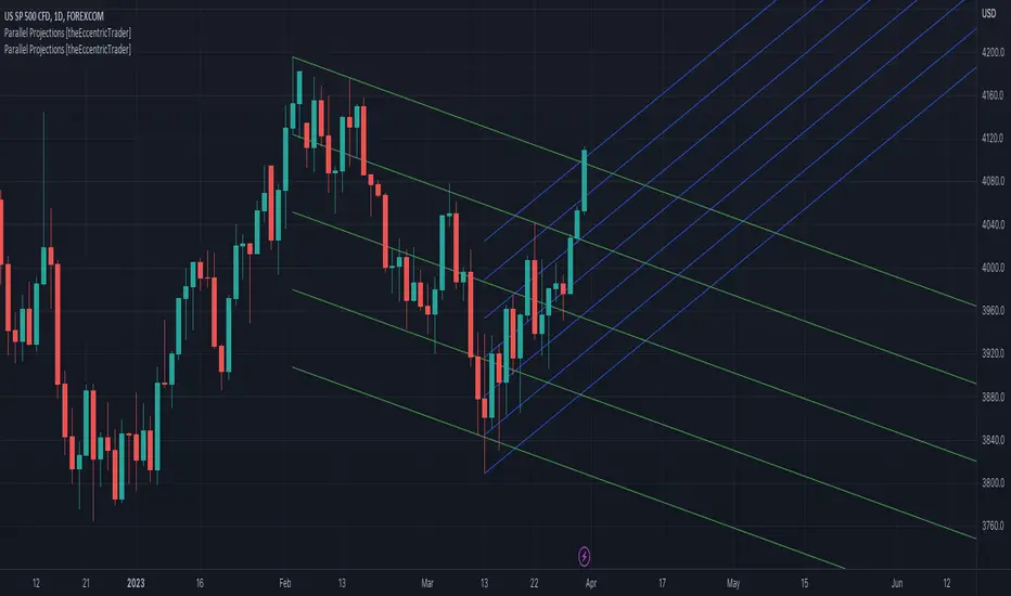
This indicator automatically projects parallel trendlines or channels, from a single point of origin. In the example above I have applied the indicator twice to the 1D SPXUSD. The five upper lines (green) are projected at an angle of -5 from the 1-month swing high anchor point with a projection ratio of -72. And the seven lower lines (blue) are projected at an angle of 10 with a projection ratio of 36 from the 1-week swing low anchor point.
█ CONCEPTS
Green and Red Candles
• A green candle is one that closes with a high price equal to or above the price it opened.
• A red candle is one that closes with a low price that is lower than the price it opened.
Swing Highs and Swing Lows
• A swing high is a green candle or series of consecutive green candles followed by a single red candle to complete the swing and form the peak.
• A swing low is a red candle or series of consecutive red candles followed by a single green candle to complete the swing and form the trough.
Peak and Trough Prices (Basic)
• The peak price of a complete swing high is the high price of either the red candle that completes the swing high or the high price of the preceding green candle, depending on which is higher.
• The trough price of a complete swing low is the low price of either the green candle that completes the swing low or the low price of the preceding red candle, depending on which is lower.
Historic Peaks and Troughs
The current, or most recent, peak and trough occurrences are referred to as occurrence zero. Previous peak and trough occurrences are referred to as historic and ordered numerically from right to left, with the most recent historic peak and trough occurrences being occurrence one.
Support and Resistance
• Support refers to a price level where the demand for an asset is strong enough to prevent the price from falling further.
• Resistance refers to a price level where the supply of an asset is strong enough to prevent the price from rising further.
Support and resistance levels are important because they can help traders identify where the price of an asset might pause or reverse its direction, offering potential entry and exit points. For example, a trader might look to buy an asset when it approaches a support level , with the expectation that the price will bounce back up. Alternatively, a trader might look to sell an asset when it approaches a resistance level , with the expectation that the price will drop back down.
It's important to note that support and resistance levels are not always relevant, and the price of an asset can also break through these levels and continue moving in the same direction.
Trendlines
Trendlines are straight lines that are drawn between two or more points on a price chart. These lines are used as dynamic support and resistance levels for making strategic decisions and predictions about future price movements. For example traders will look for price movements along, and reactions to, trendlines in the form of rejections or breakouts/downs.
█ FEATURES
Inputs
• Anchor Point Type
• Swing High/Low Occurrence
• HTF Resolution
• Highest High/Lowest Low Lookback
• Angle Degree
• Projection Ratio
• Number Lines
• Line Color
Anchor Point Types
• Swing High
• Swing Low
• Swing High (HTF)
• Swing Low (HTF)
• Highest High
• Lowest Low
• Intraday Highest High (intraday charts only)
• Intraday Lowest Low (intraday charts only)
Swing High/Swing Low Occurrence
This input is used to determine which historic peak or trough to reference for swing high or swing low anchor point types.
HTF Resolution
This input is used to determine which higher timeframe to reference for swing high (HTF) or swing low (HTF) anchor point types.
Highest High/Lowest Low Lookback
This input is used to determine the lookback length for highest high or lowest low anchor point types.
Intraday Highest High/Lowest Low Lookback
When using intraday highest high or lowest low anchor point types, the lookback length is calculated automatically based on number of bars since the daily candle opened.
Angle Degree
This input is used to determine the angle of the trendlines. The output is expressed in terms of point or pips, depending on the symbol type, which is then passed through the built in math.todegrees() function. Positive numbers will project the lines upwards while negative numbers will project the lines downwards. Depending on the market and timeframe, the impact input values will have on the visible gaps between the lines will vary greatly. For example, an input of 10 will have a far greater impact on the gaps between the lines when viewed from the 1-minute timeframe than it would on the 1-day timeframe. The input is a float and as such the value passed through can go into as many decimal places as the user requires.
It is also worth mentioning that as more lines are added the gaps between the lines, that are closest to the anchor point, will get tighter as they make their way up the y-axis. Although the gaps between the lines will stay constant at the x2 plot, i.e. a distance of 10 points between them, they will gradually get tighter and tighter at the point of origin as the slope of the lines get steeper.
Projection Ratio
This input is used to determine the distance between the parallels, expressed in terms of point or pips. Positive numbers will project the lines upwards while negative numbers will project the lines downwards. Depending on the market and timeframe, the impact input values will have on the visible gaps between the lines will vary greatly. For example, an input of 10 will have a far greater impact on the gaps between the lines when viewed from the 1-minute timeframe than it would on the 1-day timeframe. The input is a float and as such the value passed through can go into as many decimal places as the user requires.
Number Lines
This input is used to determine the number of lines to be drawn on the chart, maximum is 500.
█ LIMITATIONS
All green and red candle calculations are based on differences between open and close prices, as such I have made no attempt to account for green candles that gap lower and close below the close price of the preceding candle, or red candles that gap higher and close above the close price of the preceding candle. This may cause some unexpected behaviour on some markets and timeframes. I can only recommend using 24-hour markets, if and where possible, as there are far fewer gaps and, generally, more data to work with.
If the lines do not draw or you see a study error saying that the script references too many candles in history, this is most likely because the higher timeframe anchor point is not present on the current timeframe. This problem usually occurs when referencing a higher timeframe, such as the 1-month, from a much lower timeframe, such as the 1-minute. How far you can lookback for higher timeframe anchor points on the current timeframe will also be limited by your Trading View subscription plan. Premium users get 20,000 candles worth of data, pro+ and pro users get 10,000, and basic users get 5,000.
█ RAMBLINGS
It is my current thesis that the indicator will work best when used in conjunction with my Wavemeter indicator, which can be used to set the angle and projection ratio. For example, the average wave height or amplitude could be used as the value for the angle and projection ratio inputs. Or some factor or multiple of such an average. I think this makes sense as it allows for objectivity when applying the indicator across different markets and timeframes with different energies and vibrations.
“If you want to find the secrets of the universe, think in terms of energy, frequency and vibration.”
― Nikola Tesla
Fan Projections [theEccentricTrader]█ OVERVIEW
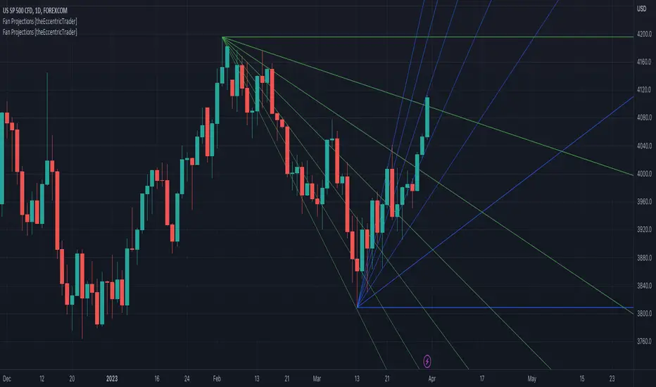
This indicator automatically projects trendlines in the shape of a fan, from a single point of origin. In the example above I have applied the indicator twice to the 1D SPXUSD. The seven upper lines (green) are projected at an angle of -5 from the 1-month swing high anchor point. And the five lower lines (blue) are projected at an angle of 10 from the 1-week swing low anchor point.
█ CONCEPTS
Green and Red Candles
• A green candle is one that closes with a high price equal to or above the price it opened.
• A red candle is one that closes with a low price that is lower than the price it opened.
Swing Highs and Swing Lows
• A swing high is a green candle or series of consecutive green candles followed by a single red candle to complete the swing and form the peak.
• A swing low is a red candle or series of consecutive red candles followed by a single green candle to complete the swing and form the trough.
Peak and Trough Prices (Basic)
• The peak price of a complete swing high is the high price of either the red candle that completes the swing high or the high price of the preceding green candle, depending on which is higher.
• The trough price of a complete swing low is the low price of either the green candle that completes the swing low or the low price of the preceding red candle, depending on which is lower.
Historic Peaks and Troughs
The current, or most recent, peak and trough occurrences are referred to as occurrence zero. Previous peak and trough occurrences are referred to as historic and ordered numerically from right to left, with the most recent historic peak and trough occurrences being occurrence one.
Support and Resistance
• Support refers to a price level where the demand for an asset is strong enough to prevent the price from falling further.
• Resistance refers to a price level where the supply of an asset is strong enough to prevent the price from rising further.
Support and resistance levels are important because they can help traders identify where the price of an asset might pause or reverse its direction, offering potential entry and exit points. For example, a trader might look to buy an asset when it approaches a support level , with the expectation that the price will bounce back up. Alternatively, a trader might look to sell an asset when it approaches a resistance level , with the expectation that the price will drop back down.
It's important to note that support and resistance levels are not always relevant, and the price of an asset can also break through these levels and continue moving in the same direction.
Trendlines
Trendlines are straight lines that are drawn between two or more points on a price chart. These lines are used as dynamic support and resistance levels for making strategic decisions and predictions about future price movements. For example traders will look for price movements along, and reactions to, trendlines in the form of rejections or breakouts/downs.
█ FEATURES
Inputs
• Anchor Point Type
• Swing High/Low Occurrence
• HTF Resolution
• Highest High/Lowest Low Lookback
• Angle Degree
• Number Lines
• Line Color
Anchor Point Types
• Swing High
• Swing Low
• Swing High (HTF)
• Swing Low (HTF)
• Highest High
• Lowest Low
• Intraday Highest High (intraday charts only)
• Intraday Lowest Low (intraday charts only)
Swing High/Swing Low Occurrence
This input is used to determine which historic peak or trough to reference for swing high or swing low anchor point types.
HTF Resolution
This input is used to determine which higher timeframe to reference for swing high (HTF) or swing low (HTF) anchor point types.
Highest High/Lowest Low Lookback
This input is used to determine the lookback length for highest high or lowest low anchor point types.
Intraday Highest High/Lowest Low Lookback
When using intraday highest high or lowest low anchor point types, the lookback length is calculated automatically based on number of bars since the daily candle opened.
Angle Degree
This input is used to determine the angle of the trendlines. The output is expressed in terms of point or pips, depending on the symbol type, which is then passed through the built in math.todegrees() function. Positive numbers will project the lines upwards while negative numbers will project the lines downwards. Depending on the market and timeframe, the impact input values will have on the visible gaps between the lines will vary greatly. For example, an input of 10 will have a far greater impact on the gaps between the lines when viewed from the 1-minute timeframe than it would on the 1-day timeframe. The input is a float and as such the value passed through can go into as many decimal places as the user requires.
It is also worth mentioning that as more lines are added the gaps between the lines, that are closest to the anchor point, will get tighter as they make their way up the y-axis. Although the gaps between the lines will stay constant at the x2 plot, i.e. a distance of 10 points between them, they will gradually get tighter and tighter at the point of origin as the slope of the lines get steeper.
Number Lines
This input is used to determine the number of lines to be drawn on the chart, maximum is 500.
█ LIMITATIONS
All green and red candle calculations are based on differences between open and close prices, as such I have made no attempt to account for green candles that gap lower and close below the close price of the preceding candle, or red candles that gap higher and close above the close price of the preceding candle. This may cause some unexpected behaviour on some markets and timeframes. I can only recommend using 24-hour markets, if and where possible, as there are far fewer gaps and, generally, more data to work with.
If the lines do not draw or you see a study error saying that the script references too many candles in history, this is most likely because the higher timeframe anchor point is not present on the current timeframe. This problem usually occurs when referencing a higher timeframe, such as the 1-month, from a much lower timeframe, such as the 1-minute. How far you can lookback for higher timeframe anchor points on the current timeframe will also be limited by your Trading View subscription plan. Premium users get 20,000 candles worth of data, pro+ and pro users get 10,000, and basic users get 5,000.
█ RAMBLINGS
It is my current thesis that the indicator will work best when used in conjunction with my Wavemeter indicator, which can be used to set the angle. For example, the average wave height or amplitude could be used as the value for the angle input. Or some factor or multiple of such an average. I think this makes sense as it allows for objectivity when applying the indicator across different markets and timeframes with different energies and vibrations.
“If you want to find the secrets of the universe, think in terms of energy, frequency and vibration.”
― Nikola Tesla
Swing Counter [theEccentricTrader]█ OVERVIEW
This indicator counts the number of confirmed swing high and swing low scenarios on any given candlestick chart and displays the statistics in a table, which can be repositioned and resized at the user's discretion.
█ CONCEPTS
Green and Red Candles
• A green candle is one that closes with a high price equal to or above the price it opened.
• A red candle is one that closes with a low price that is lower than the price it opened.
Swing Highs and Swing Lows
• A swing high is a green candle or series of consecutive green candles followed by a single red candle to complete the swing and form the peak.
• A swing low is a red candle or series of consecutive red candles followed by a single green candle to complete the swing and form the trough.
Peak and Trough Prices (Basic)
• The peak price of a complete swing high is the high price of either the red candle that completes the swing high or the high price of the preceding green candle, depending on which is higher.
• The trough price of a complete swing low is the low price of either the green candle that completes the swing low or the low price of the preceding red candle, depending on which is lower.
Peak and Trough Prices (Advanced)
• The advanced peak price of a complete swing high is the high price of either the red candle that completes the swing high or the high price of the highest preceding green candle high price, depending on which is higher.
• The advanced trough price of a complete swing low is the low price of either the green candle that completes the swing low or the low price of the lowest preceding red candle low price, depending on which is lower.
Green and Red Peaks and Troughs
• A green peak is one that derives its price from the green candle/s that constitute the swing high.
• A red peak is one that derives its price from the red candle that completes the swing high.
• A green trough is one that derives its price from the green candle that completes the swing low.
• A red trough is one that derives its price from the red candle/s that constitute the swing low.
Historic Peaks and Troughs
The current, or most recent, peak and trough occurrences are referred to as occurrence zero. Previous peak and trough occurrences are referred to as historic and ordered numerically from right to left, with the most recent historic peak and trough occurrences being occurrence one.
Upper Trends
• A return line uptrend is formed when the current peak price is higher than the preceding peak price.
• A downtrend is formed when the current peak price is lower than the preceding peak price.
• A double-top is formed when the current peak price is equal to the preceding peak price.
Lower Trends
• An uptrend is formed when the current trough price is higher than the preceding trough price.
• A return line downtrend is formed when the current trough price is lower than the preceding trough price.
• A double-bottom is formed when the current trough price is equal to the preceding trough price.
█ FEATURES
Inputs
• Start Date
• End Date
• Position
• Text Size
• Show Sample Period
• Show Plots
• Show Lines
Table
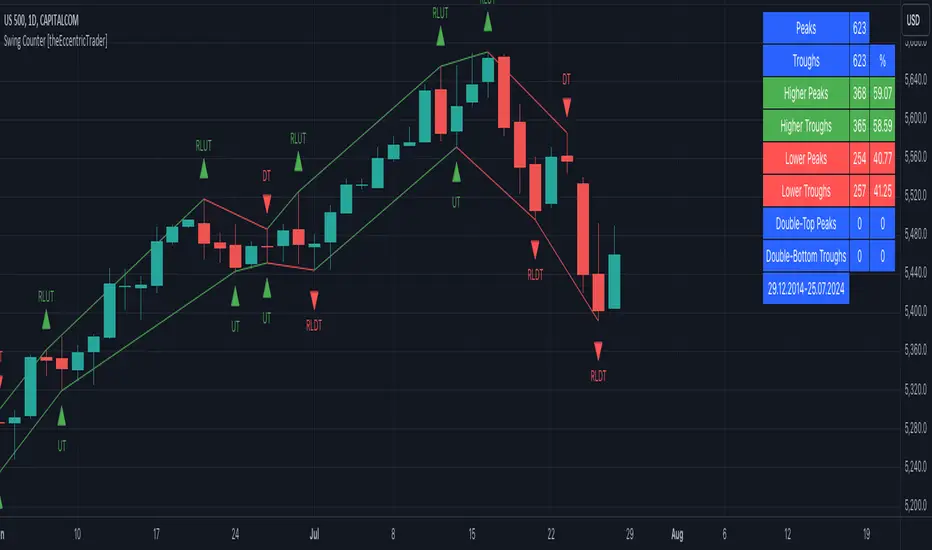
The table is colour coded, consists of three columns and nine rows. Blue cells denote neutral scenarios, green cells denote return line uptrend and uptrend scenarios, and red cells denote downtrend and return line downtrend scenarios.
The swing scenarios are listed in the first column with their corresponding total counts to the right, in the second column. The last row in column one, row nine, displays the sample period which can be adjusted or hidden via indicator settings.
Rows three and four in the third column of the table display the total higher peaks and higher troughs as percentages of total peaks and troughs, respectively. Rows five and six in the third column display the total lower peaks and lower troughs as percentages of total peaks and troughs, respectively. And rows seven and eight display the total double-top peaks and double-bottom troughs as percentages of total peaks and troughs, respectively.
Plots
I have added plots as a visual aid to the swing scenarios listed in the table. Green up-arrows with ‘HP’ denote higher peaks, while green up-arrows with ‘HT’ denote higher troughs. Red down-arrows with ‘LP’ denote higher peaks, while red down-arrows with ‘LT’ denote lower troughs. Similarly, blue diamonds with ‘DT’ denote double-top peaks and blue diamonds with ‘DB’ denote double-bottom troughs. These plots can be hidden via indicator settings.
Lines
I have also added green and red trendlines as a further visual aid to the swing scenarios listed in the table. Green lines denote return line uptrends (higher peaks) and uptrends (higher troughs), while red lines denote downtrends (lower peaks) and return line downtrends (lower troughs). These lines can be hidden via indicator settings.
█ HOW TO USE
This indicator is intended for research purposes and strategy development. I hope it will be useful in helping to gain a better understanding of the underlying dynamics at play on any given market and timeframe. It can, for example, give you an idea of any inherent biases such as a greater proportion of higher peaks to lower peaks. Or a greater proportion of higher troughs to lower troughs. Such information can be very useful when conducting top down analysis across multiple timeframes, or considering entry and exit methods.
What I find most fascinating about this logic, is that the number of swing highs and swing lows will always find equilibrium on each new complete wave cycle. If for example the chart begins with a swing high and ends with a swing low there will be an equal number of swing highs to swing lows. If the chart starts with a swing high and ends with a swing high there will be a difference of one between the two total values until another swing low is formed to complete the wave cycle sequence that began at start of the chart. Almost as if it was a fundamental truth of price action, although quite common sensical in many respects. As they say, what goes up must come down.
The objective logic for swing highs and swing lows I hope will form somewhat of a foundational building block for traders, researchers and developers alike. Not only does it facilitate the objective study of swing highs and swing lows it also facilitates that of ranges, trends, double trends, multi-part trends and patterns. The logic can also be used for objective anchor points. Concepts I will introduce and develop further in future publications.
█ LIMITATIONS
Some higher timeframe candles on tickers with larger lookbacks such as the DXY , do not actually contain all the open, high, low and close (OHLC) data at the beginning of the chart. Instead, they use the close price for open, high and low prices. So, while we can determine whether the close price is higher or lower than the preceding close price, there is no way of knowing what actually happened intra-bar for these candles. And by default candles that close at the same price as the open price, will be counted as green. You can avoid this problem by utilising the sample period filter.
The green and red candle calculations are based solely on differences between open and close prices, as such I have made no attempt to account for green candles that gap lower and close below the close price of the preceding candle, or red candles that gap higher and close above the close price of the preceding candle. I can only recommend using 24-hour markets, if and where possible, as there are far fewer gaps and, generally, more data to work with. Alternatively, you can replace the scenarios with your own logic to account for the gap anomalies, if you are feeling up to the challenge.
The sample size will be limited to your Trading View subscription plan. Premium users get 20,000 candles worth of data, pro+ and pro users get 10,000, and basic users get 5,000. If upgrading is currently not an option, you can always keep a rolling tally of the statistics in an excel spreadsheet or something of the like.
█ NOTES
I feel it important to address the mention of advanced peak and trough price logic. While I have introduced the concept, I have not included the logic in my script for a number of reasons. The most pertinent of which being the amount of extra work I would have to do to include it in a public release versus the actual difference it would make to the statistics. Based on my experience, there are actually only a small number of cases where the advanced peak and trough prices are different from the basic peak and trough prices. And with adequate multi-timeframe analysis any high or low prices that are not captured using basic peak and trough price logic on any given time frame, will no doubt be captured on a higher timeframe. See the example below on the 1H FOREXCOM:USDJPY chart (Figure 1), where the basic peak price logic denoted by the indicator plot does not capture what would be the advanced peak price, but on the 2H FOREXCOM:USDJPY chart (Figure 2), the basic peak logic does capture the advanced peak price from the 1H timeframe.
Figure 1.
Figure 2.
█ RAMBLINGS
“Never was there an age that placed economic interests higher than does our own. Never was the need of a scientific foundation for economic affairs felt more generally or more acutely. And never was the ability of practical men to utilize the achievements of science, in all fields of human activity, greater than in our day. If practical men, therefore, rely wholly on their own experience, and disregard our science in its present state of development, it cannot be due to a lack of serious interest or ability on their part. Nor can their disregard be the result of a haughty rejection of the deeper insight a true science would give into the circumstances and relationships determining the outcome of their activity. The cause of such remarkable indifference must not be sought elsewhere than in the present state of our science itself, in the sterility of all past endeavours to find its empirical foundations.” (Menger, 1871, p.45).
█ BIBLIOGRAPHY
Menger, C. (1871) Principles of Economics. Reprint, Auburn, Alabama: Ludwig Von Mises Institute: 2007.
Failed Breakdown Detection'Failed Breakdowns' are a popular set up for long entries.
In short, the set up requires:
1) A significant low is made ('initial low')
2) Initial low is undercut with a new low
3) Price action then 'reclaims' the initial low by moving +8-10 points from the initial low
This script aims at detecting such set ups. It was coded with the ES Futures 15 minute chart in mind but may be useful on other instruments and time frames.
Business Logic:
1) Uses pivot lows to detect 'significant' initial lows
2) Uses amplitude threshold to detect a new low beneath the initial low; used /u/ben_zen script for this
3) Looks for a valid reclaim - a green candle that occurs within 10 bars of the new low
4) Price must reclaim at least 8 points for the set up to be valid
5) If a signal is detected, the initial low value (pivot low) is stored in array that prevents duplicate signals from being generated.
6) FBD Signal is plotted on the chart with "X"
7) Pivot low detection is plotted on the chart with "P" and a label
8) New lows are plotted on the chart with a blue triangle
Notes:
User input
- My preference is to use the defaults as is, but as always feel free to experiment
- Can modify pivot length but in my experience 10/10 work best for pivot lows
- New low detection - 55 bars and 0.05 amplitude work well based on visual checks of signals
- Can modify the number of points needed to reclaim a low, and the # of bars limit under which this must occur.
Alerts:
- Alerts are available for detection of new lows and detection of failed breakdowns
- Alerts are also available for these signals but only during 7:30PM-4PM EST - 'prime time' US trading hours
Limitations:
- Current version of the script only compares new lows to the most recent pivot low, does not look at anything prior to that
- Best used as a discretionary signal
Visit /u/ben_zen's Profile:
www.tradingview.com
Profile Link www.tradingview.com

Price Displacement - Candlestick (OHLC) CalculationsA Magical little helper friend for Candle Math.
When composing scripts, it is often necessary to manipulate the math around the OHLC. At times, you want a scalar (absolute) value others you want a vector (+/-). Sometimes you want the open - close and sometimes you want just the positive number of the body size. You might want it in ticks or you might want it in points or you might want in percentages. And every time you try to put it together you waste precious time and brain power trying to think about how to properly structure what you're looking for. Not to mention it's normally not that aesthetically pleasing to look at in the code.
So, this fixes all of that.
Using this library. A function like 'pd.pt(_exp)' can call any kind of candlestick math you need. The function returns the candlestick math you define using particular expressions.
Candle Math Functions Include:
Points:
pt(_exp) Absolute Point Displacement. Point quantity of given size parameters according to _exp.
vpt(_exp) Vector Point Displacement. Point quantity of given size parameters according to _exp.
Ticks:
tick(_exp) Absolute Tick Displacement. Tick quantity of given size parameters according to _exp.
vtick(_exp) Vector Tick Displacement. Tick quantity of given size parameters according to _exp.
Percentages:
pct(_exp, _prec) Absolute Percent Displacement. (w/rounding overload). Percent quantity of bar range of given size parameters according to _exp.
vpct(_exp, _prec) Vector Percent Displacement (w/rounding overload). Percent quantity of bar range of given size parameters according to _exp.
Expressions You Can Use with Formulas:
The expressions are simple (simple strings that is) and I did my best to make them sensible, generally using just the ohlc abreviations. I also included uw, lw, bd, and rg for when you're just trying to pull a candle component out. That way you don't have to think about which of the ohlc you're trying to get just use pd.tick("uw") and now the variable is assigned the length of the upper wick, absolute value, in ticks. If you wanted the vector in pts its pd.vpt("uw"). It also makes changing things easy too as I write it out.
Expression List:
Combinations
"oh" = open - high
"ol" = open - low
"oc" = open - close
"ho" = high - open
"hl" = high - low
"hc" = high - close
"lo" = low - open
"lh" = low - high
"lc" = low - close
"co" = close - open
"ch" = close - high
"cl" = close - low
Candle Components
"uw" = Upper Wick
"bd" = Body
"lw" = Lower Wick
"rg" = Range
Pct() Only
"scp" = Scalar Close Position
"sop" = Scalar Open Position
"vcp" = Vector Close Position
"vop" = Vector Open Position
The attributes are going to be available in the pop up dialogue when you mouse over the function, so you don't really have to remember them. I tried to make that look as efficient as possible. You'll notice it follows the OHLC pattern. Thus, "oh" precedes "ho" (heyo) because "O" would be first in the OHLC. Its a way to help find the expression you're looking for quickly. Like looking through an alphabetized list for traders.
There is a copy/paste console friendly helper list in the script itself.
Additional Notes on the Pct() Only functions:
This is the original reason I started writing this. These concepts place a rating/value on the bar based on candle attributes in one number. These formulas put a open or close value in a percentile of the bar relative to another aspect of the bar.
Scalar - Non-directional. Absolute Value.
Scalar Position: The position of the price attribute relative to the scale of the bar range (high - low)
Example: high = 100. low = 0. close = 25.
(A) Measure price distance C-L. How high above the low did the candle close (e.g. close - low = 25)
(B) Divide by bar range (high - low). 25 / (100 - 0) = .25
Explaination: The candle closed at the 25th percentile of the bar range given the bar range low = 0 and bar range high = 100.
Formula: scp = (close - low) / (high - low)
Vector = Directional.
Vector Position: The position of the price attribute relative to the scale of the bar midpoint (Vector Position at hl2 = 0)
Example: high = 100. low = 0. close = 25.
(A) Measure Price distance C-L: How high above the low did the candle close (e.g. close - low = 25)
(B) Measure Price distance H-C: How far below the high did the candle close (e.g. high - close = 75)
(C) Take Difference: A - B = C = -50
(D) Divide by bar range (high - low). -50 / (100 - 0) = -0.50
Explaination: Candle close at the midpoint between hl2 and the low.
Formula: vcp = { / (high - low) }
Thank you for checking this out. I hope no one else has already done this (because it took half the day) and I hope you find value in it. Be well. Trade well.
Library "PD"
Price Displacement
pt(_exp) Absolute Point Displacement. Point quantity of given size parameters according to _exp.
Parameters:
_exp : (string) Price Parameter
Returns: Point size of given expression as an absolute value.
vpt(_exp) Vector Point Displacement. Point quantity of given size parameters according to _exp.
Parameters:
_exp : (string) Price Parameter
Returns: Point size of given expression as a vector.
tick(_exp) Absolute Tick Displacement. Tick quantity of given size parameters according to _exp.
Parameters:
_exp : (string) Price Parameter
Returns: Tick size of given expression as an absolute value.
vtick(_exp) Vector Tick Displacement. Tick quantity of given size parameters according to _exp.
Parameters:
_exp : (string) Price Parameter
Returns: Tick size of given expression as a vector.
pct(_exp, _prec) Absolute Percent Displacement (w/rounding overload). Percent quantity of bar range of given size parameters according to _exp.
Parameters:
_exp : (string) Expression
_prec : (int) Overload - Place value precision definition
Returns: Percent size of given expression as decimal.
vpct(_exp, _prec) Vector Percent Displacement (w/rounding overload). Percent quantity of bar range of given size parameters according to _exp.
Parameters:
_exp : (string) Expression
_prec : (int) Overload - Place value precision definition
Returns: Percent size of given expression as decimal.

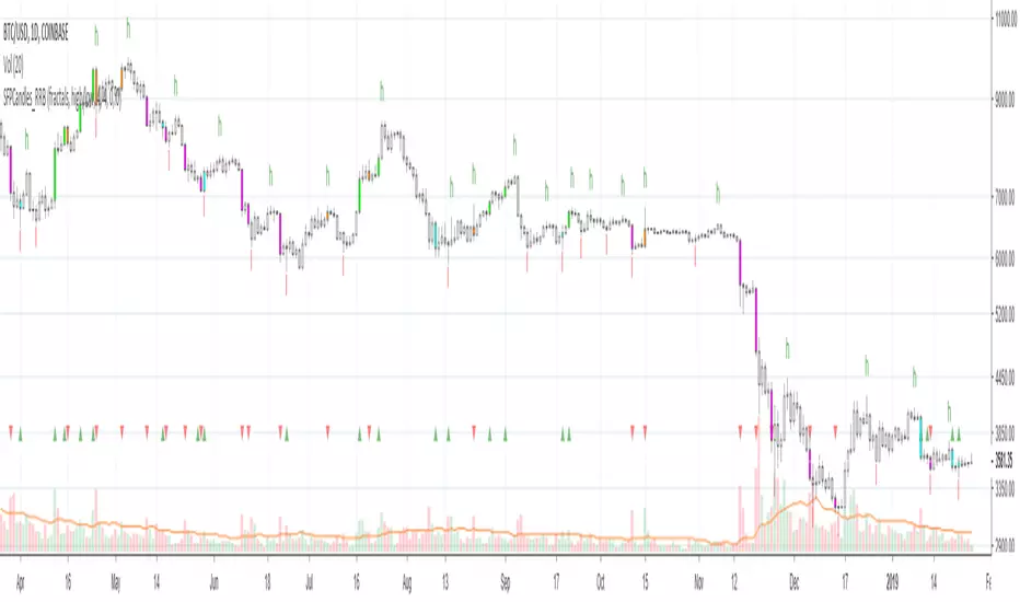
Kawabunga Swing Failure Points Candles (SFP) by RRBKawabunga Swing Failure Points Candles (SFP) by RagingRocketBull 2019
Version 1.0
This indicator shows Swing Failure Points (SFP) and Swing Confirmation Points (SCP) as candles on a chart.
SFP/SCP candles are used by traders as signals for trend confirmation/possible reversal.
The signal is stronger on a higher volume/larger candle size.
A Swing Failure Point (SFP) candle is used to spot a reversal:
- up trend SFP is a failure to close above prev high after making a new higher high => implies reversal down
- down trend SFP is a failure to close below prev low after making a new lower low => implies reversal up
A Swing Confirmation Point (SCP) candle is just the opposite and is used to confirm the current trend:
- up trend SCP is a successful close above prev high after making a new higher high => confirms the trend and implies continuation up
- down trend SCP is a successful close below prev low after making a new lower low => confirms the trend and implies continuation down
Features:
- uses fractal pivots with optional filter
- show/hide SFP/SCP candles, pivots, zigzag, last min/max pivot bands
- dim lag zones/hide false signals introduced by lagging fractals or
- use unconfirmed pivots to eliminate fractal lag/false signals. 2 modes: fractals 1,1 and highest/lowest
- filter only SFP/SCP candles confirmed with volume/candle size
- SFP/SCP candles color highlighting, dim non-important bars
Usage:
- adjust fractal settings to get pivots that best match your data (lower values => more frequent pivots. 0,0 - each candle is a pivot)
- use one of the unconfirmed pivot modes to eliminate false signals or just ignore all signals in the gray lag zones
- optionally filter only SFP/SCP candles with large volume/candle size (volume % change relative to prev bar, abs candle body size value)
- up/down trend SCP (lime/fuchsia) => continuation up/down; up/down trend SFP (orange/aqua) => possible reversal down/up. lime/aqua => up; fuchsia/orange => down.
- when in doubt use show/hide pivots/unconfirmed pivots, min/max pivot bands to see which prev pivot and min/max value were used in comparisons to generate a signal on the following candle.
- disable offset to check on which bar the signal was generated
Notes:
Fractal Pivots:
- SFP/SCP candles depend on fractal pivots, you will get different signals with different pivot settings. Usually 4,4 or 2,2 settings are used to produce fractal pivots, but you can try custom values that fit your data best.
- fractal pivots are a mixed series of highs and lows in no particular order. Pivots must be filtered to produce a proper zigzag where ideally a high is followed by a low and another high in orderly fashion.
Fractal Lag/False Signals:
- only past fractal pivots can be processed on the current bar introducing a lag, therefore, pivots and min/max pivot bands are shown with offset=-rightBars to match their target bars. For unconfirmed pivots an offset=-1 is used with a lag of just 1 bar.
- new pivot is not a confirmed fractal and "does not exist yet" while the distance between it and the current bar is < rightBars => prev old fractal pivot in the same dir is used for comparisons => gives a false signal for that dir
- to show false signals enable lag zones. SFP/SCP candles in lag zones are false. New pivots will be eventually confirmed, but meanwhile you get a false signal because prev pivot in the same dir was used instead.
- to solve this problem you can either temporary hide false signals or completely eliminate them by using unconfirmed pivots of a smaller degree/lag.
- hiding false signals only works for history and should be used only temporary (left disabled). In realtime/replay mode it disables all signals altogether due to TradingView's bug (barcolor doesn't support negative offsets)
Unconfirmed Pivots:
- you have 2 methods to check for unconfirmed pivots: highest/lowest(rightBars) or fractals(1,1) with a min possible step. The first is essentially fractals(0,0) where each candle is a pivot. Both produce more frequent pivots (weaker signals).
- an unconfirmed pivot is used in comparisons to generate a valid signal only when it is a higher high (> max high) or a lower low (< min low) in the dir of a trend. Confirmed pivots of a higher degree are not affected. Zigzag is not affected.
- you can also manually disable the offset to check on which bar the pivot was confirmed. If the pivot just before an SCP/SFP suddenly jumps ahead of it - prev pivot was used, generating a false signal.
- last max high/min low bands can be used to check which value was used in candle comparison to generate a signal: min(pivot min_low, upivot min_low) and max(pivot max_high, upivot max_high) are used
- in the unconfirmed pivots mode the max high/min low pivot bands partially break because you can't have a variable offset to match the random pos of an unconfirmed pivot (anywhere in 0..rightBars from the current bar) to its target bar.
- in the unconfirmed pivots mode h (green) and l (red) pivots become H and L, and h (lime) and l (fuchsia) are used to show unconfirmed pivots of a smaller degree. Some of them will be confirmed later as H and L pivots of a higher degree.
Pivot Filter:
- pivot filter is used to produce a better looking zigzag. Essentially it keeps only higher highs/lower lows in the trend direction until it changes, skipping:
- after a new high: all subsequent lower highs until a new low
- after a new low: all subsequent higher lows until a new high
- you can't filter out all prev highs/lows to keep just the last min/max pivots of the current swing because they were already confirmed as pivots and you can't delete/change history
- alternatively you could just pick the first high following a low and the first low following a high in a sequence and ignore the rest of the pivots in the same dir, producing a crude looking zigzag where obvious max high/min lows are ignored.
- pivot filter affects SCP/SFP signals because it skips some pivots
- pivot filter is not applied to/not affected by the unconfirmed pivots
- zigzag is affected by pivot filter, but not by the unconfirmed pivots. You can't have both high/low on the same bar in a zigzag. High has priority over Low.
- keep same bar pivots option lets you choose which pivots to keep when there are both high/low pivots on the same bar (both kept by default)
SCP/SFP Filters:
- you can confirm/filter only SCP/SFP signals with volume % change/candle size larger than delta. Higher volume/larger candle means stronger signal.
- technically SCP/SFP is always the first matching candle, but it can be invalidated by the following signal in the opposite dir which in turn can be negated by the next signal.
- show first matching SCP/SFP = true - shows only the first signal candle (and any invalidations that follow) and hides further duplicate signals in the same dir, does not highlight the trend.
- show first matching SCP/SFP = false - produces a sequence of candles with duplicate signals, highlights the whole trend until its dir changes (new pivot).
Good Luck! Feel free to learn from/reuse the code to build your own indicators!
Bollinger Bands Delta Matrix Analytics [BDMA] Bollinger Bands Delta Matrix Analytics (BDMA) v7.0
Deep Kinetic Engine – 5x8 Volatility & Delta Decision Matrix
1. Introduction & Concept
Bollinger Bands Delta Matrix Analytics (BDMA) v7.0 is an analytical framework that merges:
- Spatial analysis via Bollinger Bands (%B location),
- with a 4-factor Deep Kinetic Engine based on:
• Total Volume
• Buy Volume
• Sell Volume
• Delta (Buy – Sell) Z-Scores
and converts them into an expanded 5×8 decision matrix that continuously tracks where price is trading and how the underlying orderflow is behaving.
BDMA is not a trading system or strategy. It does not generate entry/exit signals.
Instead, it provides a structured contextual map of volatility, volume, and delta so traders can:
- identify climactic extensions vs. fakeouts,
- distinguish strong initiative moves vs. passive absorption,
- and detect squeezes, traps, and liquidity voids with a unified visual dashboard.
2. Spatial Engine – Bollinger S-States (S1–S5)
The spatial dimension of BDMA comes from classic Bollinger Bands.
Price location is expressed as Percent B (%B) and mapped into 5 spatial states (S-States):
S1 – Hyper Extension (Above Upper Band)
Price has pushed beyond the upper Bollinger Band.
Often associated with parabolic or blow-off behavior, late-stage momentum, and elevated reversal risk.
S2 – Resistance Test (Upper Zone)
Price trades in the upper Bollinger region but remains inside the bands.
Represents a sustained test of resistance, typically within an established or emerging uptrend.
S3 – Neutral Zone (Middle)
Price hovers around the mid-band.
This is the mean reversion gravity field where the market often consolidates or transitions between regimes.
S4 – Support Test (Lower Zone)
Price trades in the lower Bollinger region but inside the bands.
Represents a sustained test of support within range or downtrend structures.
S5 – Hyper Drop (Below Lower Band)
Price extends below the lower Bollinger Band.
Often aligned with panic, forced liquidations, or capitulation-type behavior, with increased snap-back risk.
These 5 S-States define the vertical axis (rows) of the BDMA matrix.
3. Deep Kinetic Engine – 4-Factor Z-Score & D-States (D1–D8)
The Deep Kinetic Engine transforms raw volume and delta into standardized Z-Scores to measure how abnormal current activity is relative to its recent history.
For each bar:
- Raw Buy Volume is estimated from the candle’s position within its range
- Raw Sell Volume is complementary to buy volume
- Raw Delta = Buy Volume – Sell Volume
- Total Volume = Buy Volume + Sell Volume
These 4 series are then normalized using a unified Z-Score lookback to produce:
1. Z_Vol_Total – overall activity and liquidity intensity
2. Z_Vol_Buy – aggression from buyers (attack)
3. Z_Vol_Sell – aggression from sellers (defense or attack)
4. Z_Delta – net victory of one side over the other
Thresholds for Extreme, Significant, and Neutral Z-Score levels are fully configurable, allowing you to tune the sensitivity of the kinetic states.
Using Z_Vol_Total and Z_Delta (plus threshold logic), BDMA assigns one of 8 Deep Kinetic states (D-States):
D1 – Climax Buy
Extreme Total Volume + Extreme Positive Delta → Buying climax or blow-off behavior.
D2 – Strong Buy
High Volume + High Positive Delta → Confirmed bullish initiative activity.
D3 – Weak Buy / Fakeout
Low Volume + High Positive Delta → Bullish delta without commitment, low-liquidity breakout risk.
D4 – Absorption / Conflict
High Volume + Neutral Delta → Aggressive two-way trade, strong absorption, war zone behavior.
D5 – Neutral
Low Volume + Neutral Delta → Low-energy environment with low conviction.
D6 – Weak Sell / Fakeout
Low Volume + High Negative Delta → Bearish delta without commitment, low-liquidity breakdown risk.
D7 – Strong Sell
High Volume + High Negative Delta → Confirmed bearish initiative activity.
D8 – Capitulation
Extreme Volume + Extreme Negative Delta → Panic selling or capitulation regime.
These 8 D-States define the horizontal axis (columns) of the BDMA matrix.
4. The 5×8 BDMA Decision Matrix
The core of BDMA is a 5×8 matrix where:
- Rows (1–5) = Spatial S-States (S1…S5)
- Columns (1–8) = Kinetic D-States (D1…D8)
Each of the 40 possible combinations (SxDy) is pre-computed and mapped to:
- a Status or Regime Title (for example: Climax Breakout, Bear Trap Spring, Capitulation Breakdown),
- a Bias (Climactic Bull, Neutral, Strong Bear, Conflict or Reversal Risk, and similar labels),
- and a Strategic Signal or Consideration (for example: High reversal risk, Wait for confirmation, Low probability zone – avoid).
Internally, BDMA resolves all 40 regimes so the current state can be displayed on the dashboard without performance overhead.
5. Key Regime Families (How to Read the Matrix)
5.1. Breakouts and Breakdowns
Climax Breakout (Top-side)
Spatial S1 with Kinetic D1 or D2
Bias: Explosive or Extreme Bull
Signal:
- Strong or climactic upside extension with abnormal bullish orderflow.
- Trend continuation is possible, but reversal risk is extremely high after blow-off phases.
Low-Conviction Breakout (Fakeout Risk)
S1 with D3 (Weak Buy, low liquidity)
Bias: Weak Bull – Caution
Signal:
- Breakout not supported by volume.
- Elevated risk of failed auction or bull trap.
Capitulation Breakdown (Bottom-side)
Spatial S5 with Kinetic D8
Bias: Climactic Bear (panic)
Signal:
- Capitulation-type selling or forced liquidations.
- Trend can still proceed, but snap-back or violent short-covering risk is high.
Initiative Breakdown vs. Weak Breakdown
- Strong, high-volume breakdown typically corresponds to D7 (Strong Sell).
- Low-volume breakdown often corresponds to D6 (Weak Sell or Fakeout) with potential for failure.
5.2. Absorption, Traps and Springs
Absorption at Resistance (Top-side conflict)
S1 or S2 with D4 (Absorption or Conflict)
Bias: Conflict – Extreme Tension
Signal:
- Heavy two-way trade near resistance.
- Potential distribution or reversal if sellers begin to dominate.
Bull Trap or Failed Auction
Typically S1 with D6 (Weak Sell breakdown behavior after a top-side attempt)
Indicates a breakout attempt that fails and reverses, often after poor liquidity structure.
Absorption at Support and Bear Trap (Spring)
S4 or S5 with D4 or D3
Bias: Conflict or Weak Bear – Reversal Risk
Signal:
- Aggressive buying into lows (spring or shakeout behavior).
- Potential bear trap if price reclaims lost territory.
5.3. Trend Phases
Strong Uptrend Phases
Typically seen when S2–S3 combine with strong bullish kinetic behavior.
Bias: Strong or Extreme Bull
Signal:
- Pullbacks into S3 or S4 with supportive kinetic states often act as trend continuation zones.
Strong Downtrend Phases
Typically seen when S3–S4 combine with strong bearish kinetic behavior.
Bias: Strong or Extreme Bear
Signal:
- Rallies into resistance with strong bearish kinetic backing may act as continuation sell zones.
5.4. Neutral, Exhaustion and Squeeze
Exhaustion or Liquidity Void
S1 or S5 with D5 (Neutral kinetics)
Bias: Neutral or Exhaustion
Signal:
- Spatial extremes without kinetic confirmation.
- Often marks the end of a move, with poor follow-through.
Choppy, Low-Activity Range
S3 with D5
Bias: Neutral
Signal:
- Low volume, low conviction market.
- Typically a low-probability environment where standing aside can be logical.
Squeeze or High-Tension Zone
S3 with D4 or tightly clustered kinetic values
Bias: Conflict or High Tension
Signal:
- Hidden battle inside a volatility contraction.
- Often precedes large directionally-biased moves.
6. Dashboard Layout & Reading Guide
When Show Dashboard is enabled, BDMA displays:
1. Title and Status Line
Name of the current regime (for example: Climax Breakout, Bear Trap Spring, Mean Reversion).
2. Bias Line
Plain-language summary of directional context such as Climactic Bull, Strong Bear, Neutral, or Conflict and Reversal Risk.
3. Signal or Strategic Notes
Concise guidance focused on risk and context, not entries. For example:
- High reversal risk – aggressive traders only
- Wait for confirmation (break or rejection)
- Low probability zone – avoid taking new positions
4. Kinetic Profile (4-Factor Z-Score)
Shows the current Z-Scores for Total Volume (Activity), Buy Volume (Attack), Sell Volume (Defense), and Delta (Net Result).
5. Matrix Heatmap (5×8)
Visual representation of S-State vs. D-State with color coding:
- Bullish clusters in a green spectrum
- Bearish clusters in a red spectrum
- Conflict or exhaustion zones in yellow, amber, or neutral tones
The dashboard can be repositioned (top right, middle right, or bottom right) and its size can be adjusted (Tiny, Small, Normal, or Large) to fit different layouts.
7. Inputs & Customization
7.1. Core Parameters (Bollinger and Z-Score)
- Bollinger Length and Standard Deviation define the spatial engine.
- Z-Score Lookback (All Factors) defines how many bars are used to normalize volume and delta.
7.2. Deep Kinetic Thresholds
- Extreme Threshold defines what is considered climactic (D1 or D8).
- Significant Threshold distinguishes strong initiative vs. weak or fakeout behavior.
- Neutral Threshold is the band within which delta is treated as neutral.
These thresholds allow you to tune the sensitivity of the kinetic classification to fit different timeframes or instruments.
7.3. Calculation Method (Volume Delta)
Geometry (Approx)
- Fast, non-repainting approach based on candle geometry.
- Suitable for most users and real-time decision-making.
Intrabar (Precise)
- Uses lower-timeframe data for more precise volume delta estimation.
- Intrabar mode can repaint and requires compatible data and plan support on the platform.
- Best used for post-analysis or research, not blind automation.
7.4. Visuals and Interface
- Toggle Bollinger Bands visibility on or off.
- Switch between Dark and Light color themes.
- Configure dashboard visibility, matrix heatmap display, position, and size.
8. Multi-Language Semantic Engine (Asia and Middle East Focus)
BDMA v7.0 includes a fully integrated multi-language layer, targeting a wide geographic user base.
Supported Languages:
English, Türkçe, Русский, 简体中文, हिन्दी, العربية, فارسی, עברית
All dashboard labels, regime titles, bias descriptions, and signal texts are dynamically translated via an internal dictionary, while semantic meaning is kept consistent across languages.
This makes BDMA suitable for multi-language communities, study groups, and educational content across different regions.
However, due to the heavy computational load of the Deep Kinetic Engine and TradingView’s strict Pine Script execution limits, it was not possible to expand support to additional languages. Adding more translation layers would significantly increase memory usage and exceed runtime constraints. For this reason, the current language set represents the maximum optimized configuration achievable without compromising performance or stability.
9. Practical Usage Notes
BDMA is most powerful when used as a contextual overlay on top of market structure (HH, HL, LH, LL), higher-timeframe trend, key levels, and your own execution framework.
Recommended usage:
- Identify the current regime (Status and Bias).
- Check whether price location (S-State) and kinetic behavior (D-State) agree with your trade idea.
- Be especially cautious in climactic and absorption or conflict zones, where volatility and risk can be elevated.
Avoid treating BDMA as an automatic green equals buy, red equals sell tool.
The real edge comes from understanding where you are in the volatility or kinetic spectrum, not from forcing signals out of the matrix.
10. Limitations & Important Warnings
BDMA does not predict the future.
It organizes current and recent data into a structured context.
Volume data quality depends on the underlying symbol, exchange, and broker feed.
Forex, crypto, indices, and stocks may all behave differently.
Intrabar mode can repaint and is sensitive to lower-timeframe data availability and your plan type.
Use it with extra caution and primarily for research.
No indicator can remove the need for clear trading rules, disciplined risk management, and psychological control.
11. Disclaimer
This script is provided strictly for educational and analytical purposes.
It is not a trading system, signal service, financial product, or investment advice.
Nothing in this indicator or its description should be interpreted as a recommendation to buy or sell any asset.
Past behavior of any indicator or market pattern does not guarantee future results.
Trading and investing involve significant risk, including the risk of losing more than your initial capital in leveraged products.
You are solely responsible for your own decisions, risk management, and results.
By using this script, you acknowledge that you understand these risks and agree that the author or authors and publisher or publishers are not liable for any loss or damage arising from its use.

The Strat Lite [rdjxyz]◆ OVERVIEW
The Strat Lite is a stripped down version of the Strat Assistant indicator by rickyzcarroll—focusing on visual simplicity and script performance. If you're new to The Strat, you may prefer the Strat Assistant as a learning aid.
◇ FEATURES REMOVED FROM THE ORIGINAL SCRIPT
Candle Numbering & Up/Down Arrows
Previous Week High & Low Lines
Previous Day High & Low Lines
Action Wick Percentage
Actionable Signals Plot
Strat Combo Plots
Extensive Alerts
◇ FEATURES KEPT FROM THE ORIGINAL SCRIPT
Full Timeframe Continuity
Candle Coloring
◇ FEATURES ADDED TO THE ORIGINAL SCRIPT
Failed 2 Down Classification
Failed 2 Up Classification
◆ DETAILS
The Strat is a trading methodology developed by Rob Smith that offers an objective approach to trading by focusing on the 3 universal scenarios regarding candle behavior:
SCENARIO ONE
The 1 Bar - Inside Bar: A candle that doesn't take out the highs or the lows of the previous candle; aka consolidation.
These are shown as gray candles by default.
SCENARIO TWO
The 2 Bar - Directional Bar: A candle that takes out one side of the previous candle; aka trending (or at least attempting to trend).
SCENARIO THREE
The 3 Bar - Outside Bar: A candle that takes out both sides of the previous candle; aka broadening formation.
In addition to Rob's 3 universal scenarios, this indicator identifies two variations of 2 bars:
Failed 2 up: A candle that takes out the high of the previous candle but closes bearish.
Failed 2 down: A candle that takes out the low of the previous candle but closes bullish.
◆ SETTINGS
◇ INPUTS
FTC (FULL TIMEFRAME CONTINUITY)
Show/hide FTC plots
Offset FTC plots from current bar
◇ STYLE
STRAT COLORS
Color 0 (Failed 2 Up) - Default is fuchsia
Color 1 (Failed 2 Down) - Default is teal
Color 2 (Inside 1) - Default is gray
Color 3 (Outside 3) - Default is dark purple
Color 4 (2 up) - Default is aqua
Color 5 (2 down) - Default is white
◆ USAGE
It's recommended to use The Strat Lite with a top down analysis so you can find lower timeframe positions with higher timeframe context.
◇ TOP DOWN ANALYSIS
MONTHLY LEVELS
Starting on a monthly chart, the previous month's high and low are manually plotted.
WEEKLY LEVELS
Dropping down to a weekly chart, the previous week's high and low are manually plotted.
DAILY LEVELS
Dropping down to a daily chart, the previous day's high and low are manually plotted.
12H LEVELS
Dropping down to a 12h chart, the previous 12h's high and low are manually plotted.
ANALYSIS
The monthly low was broken, creating a lower low (aka a broadening formation), signalling potential exhaustion risk, which can be a catalyst for reversals. The daily candle that tested the monthly low closed as a Failed 2 Down—potentially an early sign of a reversal. With these 2 confluences, it's reasonable to expect the next daily candle to be a 2 Up. Now it's time to look for a lower timeframe entry.
◇ LOWER TIMEFRAME POSITION
HOURLY PRICE ACTION
Dropping down to an hourly chart, we're anticipating a 2 Up on the daily timeframe, so we're looking for a bullish pattern to enter a position long. I personally like the 6:00 AM UTC-5 hourly candle, as it's the midpoint of the day (for futures).
In this specific example, we see the opening gap was filled and there's a potential 2-1-2 bullish reversal set up.
At this point, price can either do one of 5 things:
Form another 1 (inside) candle
Form a 2 up (directional) candle
Form a 2 down (directional) candle
Form a 2 up, fail, and potentially flip to form a bearish 3 (outside) candle
Form a 2 down, fail, and potentially flip to form a bullish 3 (outside) candle
Knowing the finite potential outcomes helps us set up our positions, manage them accordingly, and flip bias if needed.
POSITION SETUP
Here we can set up a position long AND short. To go long, we set a buy stop at the 1h high and stop loss just below the 50% level of the inside candle; to go short, we set a sell stop at 1h low and stop loss just above the 50% level of the inside candle.
If the short gets triggered first, we can wait for price to move in our favor before cancelling the buy order. If the short becomes a failed 2 down, potentially reversing to become a bullish 3, we can either wait for the stop loss to trigger and for the long position to trigger OR we can move the buy stop to our short stop loss and move the long stop loss to the low of the 1h candle.
POSITION REFINEMENT
For an even tighter risk-to-reward, we can drop to a lower timeframe and look for setups that would be an early trigger of the 1h entry. Just know, the lower you go the more noise there is—increasing risk of getting stopped out before the 1h trigger.
Above are 30m refined entries.
In this example, the long buy stop was triggered. It closed bullish, so the sell stop order can be cancelled.
◇ TARGETS & POSITION MANAGEMENT
TARGETS
These depend on whether you intend to scalp, day trade, or swing trade, but targets are typically the highs of previous candles (when bullish) and lows of previous candles (when bearish). It's advised to be cautious of swing pivots as there's a risk of exhaustion and reversal at these levels.
In this example, the nearest target was the previous 12h high and the next target was the previous day high; if you're a swing trader, you could target previous week's high and previous month's high.
POSITION MANAGEMENT
This largely depends on your risk tolerance, but it's common to either:
Move stop loss slightly into profit
Trail stop loss behind higher highs (bullish) or lower lows (bearish)
Scale out of positions at potential pivot points, leaving a runner
Scale into positions on pullbacks on the way to target
◆ WRAP UP
As demonstrated, The Strat Lite offers a stripped down version of the Strat Assistant—making it visually simple for more experienced Strat traders. By following a top-down approach with The Strat methodology, you can find high probability setups and manage risk with relative ease.
◆ DISCLAIMER
This indicator is a tool for visual analysis and is intended to assist traders who follow The Strat methodology. As with any trading methodology, there's no guarantee of profits; trading involves a high degree of risk and you could lose all of your invested capital. The example shown is of past performance and is not indicative of future results and does not constitute and should not be construed as investment advice. All trading decisions and investments made by you are at your own discretion and risk. Under no circumstances shall the author be liable for any direct, indirect, or incidental damages. You should only risk capital you can afford to lose.

Liquidity & inducementsHi all!
This indicator will show liquidity and inducements.
I will continue to try to add different types of liquidity and inducements, at this moment it contains 6 kinds of liquidity/inducement, they are:
• Grabs
• Big grabs
• Sweeps
• Turtle soups
• Equal highs/lows (liquidity and inducement)
• BSL & SSL
And 1 type of inducement:
• Retracement
This description will contain indicator examples of each individual liquidity and inducement. They will all be with the default settings.
Settings
First you will find settings for the market structure (BOS/CHoCH/CHoCH+). Select left and right pivot lengths and if the pivots should have a label or not.
This is the base foundation of this indicator and is possible with my library 'PriceAction' ().
You will see solid lines for break of structures (BOS), change of characters (CHoCH) and change of character plus (CHoCH+).
The pivots found will be the core of this indicator and will show you when the closing price breaks it. When that happens a break of structure (BOS) or a change of character (CHoCH or CHoCH+) will be created. The latest 5 pivots found within the current trend will be kept to take action on.
A break of structure is removed if an earlier pivot within the same trend is broken and the pivot's high price for a bullish trend or low price for a bearish trend is more extreme than the BOS pivot's price.
You are able to show the pivots that are used. "HH" (higher high), "HL" (higher low), "LH" (lower high), "LL" (lower low) and "H"/"L" (for pivots (high/low) when the trend has changed) are the labels used.
In the next section ('Liquidity ($$$)') you can select which types of liquidity you want to see. Note that 'Equal highs/lows' can also show inducement (more on that later).
In the section afterwards ('Inducement (IDM)') you can select if you want retracement inducements to be visible or not. More information on what they are later on.
The section for each individual liquidity and/or inducement can first contain a line named 'Pivot', where you can set the pivot lengths (first left, then right). Then you can set the 'Lookback', which means that the 'Lookback' number of past pivots is to take action on. After that you set the 'Timeframe' for the pivots used. That means that all available liquidity/inducements will be from your desired timeframe. Lastly you set the color of the liquidity/inducement (either a single color or bullish followed by bearish colors).
Lastly in the settings you can select the font sizes for the market structure and liquidity/inducements and what style liquidity/inducements lines will have. The sizes defaults to 7 and has a dotted line look.
Grabs
Liquidity grabs and liquidity sweeps are very similar. It all depends on if the current bar closed above/below the liquidity pivot and on if its a continuation or reversal. In a liquidity grab the bar that's above or below the liquidity pivot was not closed above or below it. Like this:
Or
The visual feedback will be a dotted line between the liquidity pivot and liquidity grab bar and a linefill between the high of the liquidity grab bar and the liquidity pivot.
Indicator example:
Big grabs
This is another 'grabs' option. You can show an additional grab if you want to. I suggest having this grab from a higher timeframe or with larger pivot lengths than the other grab.
The default is with the chart timeframe and 10/10 as pivot lengths.
Indicator example:
Sweeps
A liquidity sweep is like a liquidity grab but with the difference that price closes above/below and has a continuation instead of a reversal. If the liquidity pivot was at the same bar as a BOS/CHoCH/CHoCH+ it will not be a liquidity grab but a structural break instead.
They can look like this:
Indicator example;
Turtle soups
If only one candle is beyond the pivot it could be a liquidity grab. It's a grab if price didn't close beyond the liquidity pivot, if so it's invaliditet. Turtle soups are basically false breakouts that takes liquidity (is a false breakout from a pivot with the lengths and timeframe from the settings).
The turtle soup can have a confirmation in the terms of a change of character (CHoCH). You can enable this in the settings section for 'Turtle soups' through the 'Confirmation' checkbox (enabled by default). The turtle soup strategy usually comes with some sort of confirmation, in this case a CHoCH, but it can also be a market structure shift (MSS) or a change in state of delivery (CISD).
The addition of turtle soups is possible through my script 'Turtle soup' ().
The drawing will be a dotted line between the liquidity pivot and the last bar of the false breakout and a box from the start of the false breakout to the end of it.
Indicator example:
Equal highs/lows
Equal highs/lows will always show liquidity, but might also show inducement. Inducement will be shown on equal lows if the trend is bullish and on equal highs if it's bearish, like this:
Or
Equal highs can only be created if the second pivot is lower than the first one. Equal lows can only be created if the second pivot is higher than the first one. If that is not the case it could be a liquidity grab.
When equal highs or equal lows are find that produces inducement (equal lows in a bullish trend and equal highs in a bearish trend), the indicator will first display inducement and will show liquidity once traders are induced to enter the security. Stop loss placement, for liquidity, is 0.1 * the average true range (ATR, of length 14). They will look like this:
Only inducement:
Inducement and liquidity:
Indicator example:
Equal highs/lows inducements can not be triggered after a BOS/CHoCH/CHoCH+. They are cleared upon a structural break.
BSL & SSL
Buyside liquidity (BSL) and sellside liquidity (SSL) will be shown. A pivot that's been mitigated (touched by price) can never be BSL or SSL. The BSL/SSL available will be dynamic while price moves (work in Replay and lower timeframes that moves fast) and pick the latest pivot/s (with left and right lengths from the 'Market structure' section). You can define how many BSL/SSL you want to see with a default value of 1, meaning only 1 BSL and 1 SSL can be shown. If there is no unmitigated high (BSL) or low (SSL), no BSL/SSL will be available to show. If there are BSL/SSL available they're very useful to use as targets for entering a trade.
The will look like this when available;
And without BSL available:
Or
And without SSL available:
Note that the examples without BSL/SSL available could have liquidity available from previous price legs.
This can be an example of a BSL/SSL sequence:
First both buyside and sellside liquidity is available:
Then a new low appears and new sellside liquidity is available:
Then buyside liquidity is mitigated, so only sellside liquidity is available:
A new high pivot appears and buyside liquidity is available again:
Lastly a bearish CHoCH happens and sellside liquidity is mitigated, only buyside liquidity is available:
Retracement
The first retracement after a BOS/CHoCH/CHoCH+ is considered an inducement with the mission to get traders into a trade prematurely to get stopped out. This level is shown and look like this:
Or
A retracement inducement is removed when a new BOS/CHoCH/CHoCH+ appears and it's not triggered.
---------------------------
As of now there aren't any alerts available. You cannot use the Pine Screener from Tradingview either to see new liquidity/inducement events. I have this planned for future updates though.
I hope that this long description makes sense, let me know otherwise! Also let me know if you experience any bugs or have a feature request or just want to share good settings to use.
Best of trading luck!

Pivot Regime Anchored VWAP [CHE] Pivot Regime Anchored VWAP — Detects body-based pivot regimes to classify swing highs and lows, anchoring volume-weighted average price lines directly at higher highs and lower lows for adaptive reference levels.
Summary
This indicator identifies shifts between top and bottom regimes through breakouts in candle body highs and lows, labeling swing points as higher highs, lower highs, lower lows, or higher lows. It then draws anchored volume-weighted average price lines starting from the most recent higher high and lower low, providing dynamic support and resistance that evolve with volume flow. These anchored lines differ from standard volume-weighted averages by resetting only at confirmed swing extremes, reducing noise in ranging markets while highlighting momentum shifts in trends.
Motivation: Why this design?
Traders often struggle with static reference lines that fail to adapt to changing market structures, leading to false breaks in volatile conditions or missed continuations in trends. By anchoring volume-weighted average price calculations to body pivot regimes—specifically at higher highs for resistance and lower lows for support—this design creates reference levels tied directly to price structure extremes. This approach addresses the problem of generic moving averages lagging behind swing confirmations, offering a more context-aware tool for intraday or swing trading.
What’s different vs. standard approaches?
- Baseline reference: Traditional volume-weighted average price indicators compute a running total from session start or fixed periods, often ignoring price structure.
- Architecture differences:
- Regime detection via body breakout logic switches between high and low focus dynamically.
- Anchoring limited to confirmed higher highs and lower lows, with historical recalculation for accurate line drawing.
- Polyline rendering rebuilds only on the last bar to manage performance.
- Practical effect: Charts show fewer, more meaningful lines that start at swing points, making it easier to spot confluences with structure breaks rather than cluttered overlays from continuous calculations.
How it works (technical)
The indicator first calculates the maximum and minimum of each candle's open and close to define body highs and lows. It then scans a lookback window for the highest body high and lowest body low. A top regime triggers when the body high from the lookback period exceeds the window's highest, and a bottom regime when the body low falls below the window's lowest. These regime shifts confirm pivots only when crossing from one state to the other.
For top pivots, it compares the new body high against the previous swing high: if greater, it marks a higher high and anchors a new line; otherwise, a lower high. The same logic applies inversely for bottom pivots. Anchored lines use cumulative price-volume products and volumes from the anchor bar onward, subtracting prior cumulatives to isolate the segment. On pivot confirmation, it loops backward from the current bar to the anchor, computing and storing points for the line. New points append as bars advance, ensuring the line reflects ongoing volume weighting.
Initialization uses persistent variables to track the last swing values and anchor bars, starting with neutral states. Data flows from regime detection to pivot classification, then to anchoring and point accumulation, with lines rendered globally on the final bar.
Parameter Guide
Pivot Length — Controls the lookback window for detecting body breakouts, influencing pivot frequency and sensitivity to recent action. Shorter values catch more pivots in choppy conditions; longer smooths for major swings. Default: 30 (bars). Trade-offs/Tips: Min 1; for intraday, try 10–20 to reduce lag but watch for noise; on daily, 50+ for stability.
Show Pivot Labels — Toggles display of text markers at swing points, aiding quick identification of higher highs, lower highs, lower lows, or higher lows. Default: true. Trade-offs/Tips: Disable in multi-indicator setups to declutter; useful for backtesting structure.
HH Color — Sets the line and label color for higher high anchored lines, distinguishing resistance levels. Default: Red (solid). Trade-offs/Tips: Choose contrasting hues for dark/light themes; pair with opacity for fills if added later.
LL Color — Sets the line and label color for lower low anchored lines, distinguishing support levels. Default: Lime (solid). Trade-offs/Tips: As above; green shades work well for bullish contexts without overpowering candles.
Reading & Interpretation
Higher high labels and red lines indicate potential resistance zones where volume weighting begins at a new swing top, suggesting sellers may defend prior highs. Lower low labels and lime lines mark support from a fresh swing bottom, with the line's slope reflecting buyer commitment via volume. Lower highs or higher lows appear as labels without new anchors, signaling possible range-bound action. Line proximity to price shows overextension; crosses may hint at regime shifts, but confirm with volume spikes.
Practical Workflows & Combinations
- Trend following: Enter longs above a rising lower low anchored line after higher low confirmation; filter with rising higher highs for uptrends. Use line breaks as trailing stops.
- Exits/Stops: In downtrends, exit shorts below a higher high line; set aggressive stops above it for scalps, conservative below for swings. Pair with momentum oscillators for divergence.
- Multi-asset/Multi-TF: Defaults suit forex/stocks on 1H–4H; on crypto 15M, shorten length to 15. Scale colors for dark themes; combine with higher timeframe anchors for confluence.
Behavior, Constraints & Performance
Closed-bar logic ensures pivots confirm after the lookback period, with no repainting on historical bars—live bars may adjust until regime shift. No higher timeframe calls, so minimal repaint risk beyond standard delays. Resources include a 2000-bar history limit, label/polyline caps at 200/50, and loops for historical point filling (up to current bar count from anchor, typically under 500 iterations). Known limits: In extreme gaps or low-volume periods, anchors may skew; lines absent until first pivots.
Sensible Defaults & Quick Tuning
Start with the 30-bar length for balanced pivot detection across most assets. For too-frequent pivots in ranges, increase to 50 for fewer signals. If lines lag in trends, reduce to 20 and enable labels for visual cues. In low-volatility assets, widen color contrasts; test on 100-bar history to verify stability.
What this indicator is—and isn’t
This is a structure-aware visualization layer for anchoring volume-weighted references at swing extremes, enhancing manual analysis of regimes and levels. It is not a standalone signal generator or predictive model—always integrate with broader context like order flow or news. Use alongside risk management and position sizing, not as isolated buy/sell triggers.
Many thanks to LuxAlgo for the original script "McDonald's Pattern ". The implementation for body pivots instead of wicks uses a = max(open, close), b = min(open, close) and then highest(a, length) / lowest(b, length). This filters noise from the wicks and detects breakouts over/under bodies. Unusual and targeted, super innovative.
Disclaimer
The content provided, including all code and materials, is strictly for educational and informational purposes only. It is not intended as, and should not be interpreted as, financial advice, a recommendation to buy or sell any financial instrument, or an offer of any financial product or service. All strategies, tools, and examples discussed are provided for illustrative purposes to demonstrate coding techniques and the functionality of Pine Script within a trading context.
Any results from strategies or tools provided are hypothetical, and past performance is not indicative of future results. Trading and investing involve high risk, including the potential loss of principal, and may not be suitable for all individuals. Before making any trading decisions, please consult with a qualified financial professional to understand the risks involved.
By using this script, you acknowledge and agree that any trading decisions are made solely at your discretion and risk.
Do not use this indicator on Heikin-Ashi, Renko, Kagi, Point-and-Figure, or Range charts, as these chart types can produce unrealistic results for signal markers and alerts.
Best regards and happy trading
Chervolino

Liquidity Void Detector (Zeiierman)█ Overview
Liquidity Void Detector (Zeiierman) is an oscillator highlighting inefficient price displacements under low participation. It measures the most recent price move (standardized return) and amplifies it only when volume is below its own trend.
Positive readings ⇒ strong up-move on low volume → potential Buy-Side Imbalance (void below) that often refills.
Negative readings ⇒ strong down-move on low volume → potential Sell-Side Imbalance (void above) that often refills.
This tool provides a quantitative “void” proxy: when price travels far with unusually thin volume, the move is flagged as likely inefficient and prone to mean-reversion/mitigation.
█ How It Works
⚪ Volume Shock (Participation Filter)
Each bar, volume is compared to a rolling baseline. This is then z-scored.
// Volume Shock calculation
volTrend = ta.sma(volume, L)
vs = (volume > 0 and volTrend > 0) ? math.log(volume) - math.log(volTrend) : na
vsZ = zScore(vs, vzLen) // z-scored volume shock
lowVS = (vsZ <= vzThr) // low-volume condition
Bars with VolShock Z ≤ threshold are treated as low-volume (thin).
⚪ Prior Return Extremeness
The 1-bar log return is computed and z-scored.
// Prior return extremeness
r1 = math.log(close / close )
retZ = zScore(r1, rLen) // z-scored prior return
This shows whether the latest move is unusually large relative to recent history.
⚪ Void Oscillator
The oscillator is:
// Oscillator construction
weight = lowVS ? 1.0 : fadeNoLow
osc = retZ * weight
where Weight = 1 when volume is low, otherwise fades toward a user-set factor (0–1).
Osc > 0: up-move emphasized under low volume ⇒ Buy-Side Imbalance.
Osc < 0: down-move emphasized under low volume ⇒ Sell-Side Imbalance.
█ Why Use It
⚪ Targets Inefficient Moves
By filtering for low participation, the oscillator focuses on moves most likely driven by thin books/noise trading, which are statistically more likely to retrace.
⚪ Simple, Robust Logic
No need for tick data or order-book depth. It derives a practical void proxy from OHLCV, making it portable across assets and timeframes.
⚪ Complements Price-Action Tools
Use alongside FVG/imbalance zones, key levels, and volume profile to prioritize voids that carry the highest reversal probability.
█ How to Use
Sell-Side Imbalance = aggressive sell move (price goes down on low volume) → expect price to move up to fill it.
Buy-Side Imbalance = aggressive buy move (price goes up on low volume) → expect price to move down to fill it.
█ Settings
Volume Baseline Length — Bars for the volume trend used in VolShock. Larger = smoother baseline, fewer low-volume flags.
Vol Shock Z-Score Lookback — Bars to standardize VolShock; larger = smoother, fewer extremes.
Low-Volume Threshold (VolShock Z ≤) — Defines “thin participation.” Typical: −0.5 to −1.0.
Return Z-Score Lookback — Bars to standardize the 1-bar log return; larger = smoother “extremeness” measure.
Fade When Volume Not Low (0–1) — Weight applied when volume is not low. 0.00 = ignore non-low-volume bars entirely. 1.00 = treat volume condition as irrelevant (pure return extremeness).
Upper Threshold (Osc ≥) — Trigger for Sell-Side Imbalance (void below).
Lower Threshold (Osc ≤) — Trigger for Buy-Side Imbalance (void above).
-----------------
Disclaimer
The content provided in my scripts, indicators, ideas, algorithms, and systems is for educational and informational purposes only. It does not constitute financial advice, investment recommendations, or a solicitation to buy or sell any financial instruments. I will not accept liability for any loss or damage, including without limitation any loss of profit, which may arise directly or indirectly from the use of or reliance on such information.
All investments involve risk, and the past performance of a security, industry, sector, market, financial product, trading strategy, backtest, or individual's trading does not guarantee future results or returns. Investors are fully responsible for any investment decisions they make. Such decisions should be based solely on an evaluation of their financial circumstances, investment objectives, risk tolerance, and liquidity needs.

ATR Future Movement Range Projection
The "ATR Future Movement Range Projection" is a custom TradingView Pine Script indicator designed to forecast potential price ranges for a stock (or any asset) over short-term (1-month) and medium-term (3-month) horizons. It leverages the Average True Range (ATR) as a measure of volatility to estimate how far the price might move, while incorporating recent momentum bias based on the proportion of bullish (green) vs. bearish (red) candles. This creates asymmetric projections: in bullish periods, the upside range is larger than the downside, and vice versa.
The indicator is overlaid on the chart, plotting horizontal lines for the projected high and low prices for both timeframes. Additionally, it displays a small table in the top-right corner summarizing the projected prices and the percentage change required from the current close to reach them. This makes it useful for traders assessing potential targets, risk-reward ratios, or option strategies, as it combines volatility forecasting with directional sentiment.
Key features:
- **Volatility Basis**: Uses weekly ATR to derive a stable daily volatility estimate, avoiding noise from shorter timeframes.
- **Momentum Adjustment**: Analyzes recent candle colors to tilt projections toward the prevailing trend (e.g., more upside if more green candles).
- **Time Horizons**: Fixed at 1 month (21 trading days) and 3 months (63 trading days), assuming ~21 trading days per month (excluding weekends/holidays).
- **User Adjustable**: The ATR length/lookback (default 50) can be tweaked via inputs.
- **Visuals**: Green/lime lines for highs, red/orange for lows; a semi-transparent table for quick reference.
- **Limitations**: This is a probabilistic projection based on historical volatility and momentum—it doesn't predict direction with certainty and assumes volatility persists. It ignores external factors like news, earnings, or market regimes. Best used on daily charts for stocks/ETFs.
The indicator doesn't generate buy/sell signals but helps visualize "expected" ranges, similar to how implied volatility informs option pricing.
### How It Works Step-by-Step
The script executes on each bar update (typically daily timeframe) and follows this logic:
1. **Input Configuration**:
- ATR Length (Lookback): Default 50 bars. This controls both the ATR calculation period and the candle count window. You can adjust it in the indicator settings.
2. **Calculate Weekly ATR**:
- Fetches the ATR from the weekly timeframe using `request.security` with a length of 50 weeks.
- ATR measures average price range (high-low, adjusted for gaps), representing volatility.
3. **Derive Daily ATR**:
- Divides the weekly ATR by 5 (approximating 5 trading days per week) to get an equivalent daily volatility estimate.
- Example: If weekly ATR is $5, daily ATR ≈ $1.
4. **Define Projection Periods**:
- 1 Month: 21 trading days.
- 3 Months: 63 trading days (21 × 3).
- These are hardcoded but based on standard trading calendar assumptions.
5. **Compute Base Projections**:
- Base projection = Daily ATR × Days in period.
- This gives the total expected movement (range) without direction: e.g., for 3 months, $1 daily ATR × 63 = $63 total range.
6. **Analyze Candle Momentum (Win Rate)**:
- Counts green candles (close > open) and red candles (close < open) over the last 50 bars (ignores dojis where close == open).
- Total colored candles = green + red.
- Win rate = green / total colored (as a fraction, e.g., 0.7 for 70%). Defaults to 0.5 if no colored candles.
- This acts as a simple momentum proxy: higher win rate implies bullish bias.
7. **Adjust Projections Asymmetrically**:
- Upside projection = Base projection × Win rate.
- Downside projection = Base projection × (1 - Win rate).
- This skews the range: e.g., 70% win rate means 70% of the total range allocated to upside, 30% to downside.
8. **Calculate Projected Prices**:
- High = Current close + Upside projection.
- Low = Current close - Downside projection.
- Done separately for 1M and 3M.
9. **Plot Lines**:
- 3M High: Solid green line.
- 3M Low: Solid red line.
- 1M High: Dashed lime line.
- 1M Low: Dashed orange line.
- Lines extend horizontally from the current bar onward.
10. **Display Table**:
- A 3-column table (Projection, Price, % Change) in the top-right.
- Rows for 1M High/Low and 3M High/Low, color-coded.
- % Change = ((Projected price - Close) / Close) × 100.
- Updates dynamically with new data.
The entire process repeats on each new bar, so projections evolve as volatility and momentum change.
### Examples
Here are two hypothetical examples using the indicator on a daily chart. Assume it's applied to a stock like AAPL, but with made-up data for illustration. (In TradingView, you'd add the script to see real outputs.)
#### Example 1: Bullish Scenario (High Win Rate)
- Current Close: $150.
- Weekly ATR (50 periods): $10 → Daily ATR: $10 / 5 = $2.
- Last 50 Candles: 35 green, 15 red → Total colored: 50 → Win Rate: 35/50 = 0.7 (70%).
- Base Projections:
- 1M: $2 × 21 = $42.
- 3M: $2 × 63 = $126.
- Adjusted Projections:
- 1M Upside: $42 × 0.7 = $29.4 → High: $150 + $29.4 = $179.4 (+19.6%).
- 1M Downside: $42 × 0.3 = $12.6 → Low: $150 - $12.6 = $137.4 (-8.4%).
- 3M Upside: $126 × 0.7 = $88.2 → High: $150 + $88.2 = $238.2 (+58.8%).
- 3M Downside: $126 × 0.3 = $37.8 → Low: $150 - $37.8 = $112.2 (-25.2%).
- On the Chart: Green/lime lines skewed higher; table shows bullish % changes (e.g., +58.8% for 3M high).
- Interpretation: Suggests stronger potential upside due to recent bullish momentum; useful for call options or long positions.
#### Example 2: Bearish Scenario (Low Win Rate)
- Current Close: $50.
- Weekly ATR (50 periods): $3 → Daily ATR: $3 / 5 = $0.6.
- Last 50 Candles: 20 green, 30 red → Total colored: 50 → Win Rate: 20/50 = 0.4 (40%).
- Base Projections:
- 1M: $0.6 × 21 = $12.6.
- 3M: $0.6 × 63 = $37.8.
- Adjusted Projections:
- 1M Upside: $12.6 × 0.4 = $5.04 → High: $50 + $5.04 = $55.04 (+10.1%).
- 1M Downside: $12.6 × 0.6 = $7.56 → Low: $50 - $7.56 = $42.44 (-15.1%).
- 3M Upside: $37.8 × 0.4 = $15.12 → High: $50 + $15.12 = $65.12 (+30.2%).
- 3M Downside: $37.8 × 0.6 = $22.68 → Low: $50 - $22.68 = $27.32 (-45.4%).
- On the Chart: Red/orange lines skewed lower; table highlights larger downside % (e.g., -45.4% for 3M low).
- Interpretation: Indicates bearish risk; might prompt protective puts or short strategies.
#### Example 3: Neutral Scenario (Balanced Win Rate)
- Current Close: $100.
- Weekly ATR: $5 → Daily ATR: $1.
- Last 50 Candles: 25 green, 25 red → Win Rate: 0.5 (50%).
- Projections become symmetric:
- 1M: Base $21 → Upside/Downside $10.5 each → High $110.5 (+10.5%), Low $89.5 (-10.5%).
- 3M: Base $63 → Upside/Downside $31.5 each → High $131.5 (+31.5%), Low $68.5 (-31.5%).
- Interpretation: Pure volatility-based range, no directional bias—ideal for straddle options or range trading.
In real use, test on historical data: e.g., if past projections captured actual moves ~68% of the time (1 standard deviation for ATR), it validates the volatility assumption. Adjust the lookback for different assets (shorter for volatile cryptos, longer for stable blue-chips).

Trade Calculator {Phanchai}Trade Calculator 🧮 {Phanchai} — Documentation
A lightweight sizing helper for TradingView that turns your risk per trade into an estimated maximum nominal position size — using the most recent chart low as your stop reference. Built for speed and clarity right on the chart.
Key Features
Clean on-chart info table with configurable font size and position.
Row toggles: show/hide each line (Price, Last Low, Risk per Trade, Entry − Low, SL to Low %, Max. Nominal Value in USDT).
Configurable low reference: Last N bars or Running since load .
Low label placed exactly at the wick of the lowest bar (no horizontal line).
Custom padding: add extra rows above/below and blank columns left/right (with custom whitespace/text fillers) to fine-tune layout.
Integer display for Risk per Trade (USDT) and Max. Nominal Value (USDT); decimals configurable elsewhere.
Open source script — easy to read and extend.
How to Use
Add the indicator: open TradingView → Indicators → paste the source code → Add to chart.
Pick your low reference in settings:
Last N bars — uses the lowest low within your chosen lookback.
Running since load — tracks the lowest low since the script loaded.
Set your capital and risk:
Total Capital — your account size in USDT.
Max. invest Capital per Trade (%) — your risk per trade as a percent of Total Capital.
Tidy the table:
Use Table Position and Table Size to place it.
Add Extra rows/columns and set left/right fillers (spaces allowed) for padding.
Toggle individual rows (on/off) to show only what you need.
Read the numbers:
Act. Price in USDT — current close.
Last Low in USDT — stop reference price.
Risk per Trade — whole-USDT value of your risk budget for this trade.
Entry − Low — absolute risk per unit.
SL to Low (%) — percentage distance from price to low.
Max. Nominal Value in USDT — estimated max nominal position size given your risk budget and stop at the low.
Scope
This calculator is designed for long trades only (stop below price at the chart low).
Notes & Assumptions
Does not factor fees, funding, slippage, tick size, or broker/venue position limits.
“Running since load” updates as new lows appear; “Last N bars” uses only the selected lookback window.
If price equals the low (zero distance), sizing will be undefined (division by zero guarded as “—”).
Risk Warning
Trading involves substantial risk. Always double-check every value the calculator shows, confirm your stop distance, and verify position sizing with your broker/platform before entering any order. Never risk money you cannot afford to lose.
Open Source & Feedback
The source code is open. If you spot a bug or have an idea to improve the tool, feel free to share suggestions — I’m happy to iterate and make it better.