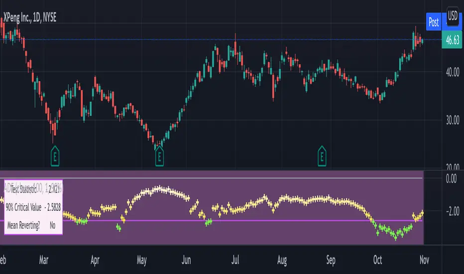
Augmented Dickey–Fuller (ADF) mean reversion testThe augmented Dickey-Fuller test (ADF) is a statistical test for the tendency of a price series sample to mean revert .
The current price of a mean-reverting series may tell us something about the next move (as opposed, for example, to a geometric Brownian motion). Thus, the ADF test allows us to spot market inefficiencies and potentially exploit this information in a trading strategy.
Mathematically, the mean reversion property means that the price change in the next time period is proportional to the difference between the average price and the current price. The purpose of the ADF test is to check if this proportionality constant is zero. Accordingly, the ADF test statistic is defined as the estimated proportionality constant divided by the corresponding standard error.
In this script, the ADF test is applied in a rolling window with a user-defined lookback length. The calculated values of the ADF test statistic are plotted as a time series. The more negative the test statistic, the stronger the rejection of the hypothesis that there is no mean reversion. If the calculated test statistic is less than the critical value calculated at a certain confidence level (90%, 95%, or 99%), then the hypothesis of a mean reversion is accepted (strictly speaking, the opposite hypothesis is rejected).
Input parameters:
Source - The source of the time series being tested.
Length - The number of points in the rolling lookback window. The larger sample length makes the ADF test results more reliable.
Maximum lag - The maximum lag included in the test, that defines the order of an autoregressive process being implied in the model. Generally, a non-zero lag allows taking into account the serial correlation of price changes. When dealing with price data, a good starting point is lag 0 or lag 1.
Confidence level - The probability level at which the critical value of the ADF test statistic is calculated. If the test statistic is below the critical value, it is concluded that the sample of the price series is mean-reverting. Confidence level is calculated based on MacKinnon (2010) .
Show Infobox - If True, the results calculated for the last price bar are displayed in a table on the left.
More formal background:
Formally, the ADF test is a test for a unit root in an autoregressive process. The model implemented in this script involves a non-zero constant and zero time trend. The zero lag corresponds to the simple case of the AR(1) process, while higher order autoregressive processes AR(p) can be approached by setting the maximum lag of p. The null hypothesis is that there is a unit root, with the alternative that there is no unit root. The presence of unit roots in an autoregressive time series is characteristic for a non-stationary process. Thus, if there is no unit root, the time series sample can be concluded to be stationary, i.e., manifesting the mean-reverting property.
A few more comments:
It should be noted that the ADF test tells us only about the properties of the price series now and in the past. It does not directly say whether the mean-reverting behavior will retain in the future.
The ADF test results don't directly reveal the direction of the next price move. It only tells wether or not a mean-reverting trading strategy can be potentially applicable at the given moment of time.
The ADF test is related to another statistical test, the Hurst exponent. The latter is available on TradingView as implemented by balipour , QuantNomad and DonovanWall .
The ADF test statistics is a negative number. However, it can take positive values, which usually corresponds to trending markets (even though there is no statistical test for this case).
Rigorously, the hypothesis about the mean reversion is accepted at a given confidence level when the value of the test statistic is below the critical value. However, for practical trading applications, the values which are low enough - but still a bit higher than the critical one - can be still used in making decisions.
Examples:
The VIX volatility index is known to exhibit mean reversion properties (volatility spikes tend to fade out quickly). Accordingly, the statistics of the ADF test tend to stay below the critical value of 90% for long time periods.
The opposite case is presented by BTCUSD. During the same time range, the bitcoin price showed strong momentum - the moves away from the mean did not follow by the counter-move immediately, even vice versa. This is reflected by the ADF test statistic that consistently stayed above the critical value (and even above 0). Thus, using a mean reversion strategy would likely lead to losses.
Wyszukaj w skryptach "hurst"
AMF PG Strategy v2.3AMF PG Strategy v2.3
1. Core Philosophy: Filtered and Volatility-Aware Trend Following
"AMF PG Strategy" is an advanced trend-following system designed to adapt to the dynamic nature of modern markets. The strategy's core philosophy is not just to follow the trend but also to wait for the right conditions to enter the market.
This is not a "black box." It is a rules-based framework that gives the user full control over various market filters. By requiring multiple conditions to be met simultaneously, the strategy aims to filter out low-quality signals and focus only on high-probability trend opportunities.
2. Core Engine: AMF PG Trend Following
At the heart of the strategy is a proprietary, volatility-aware trend-following mechanism called AMF PG (Praetorian Guard). This engine operates as follows:
Dynamic Bands: Creates a dynamic upper and lower band around the price that is constantly recalculated. The width of these bands is not fixed; It dynamically adjusts based on recent market volatility, volume flow, and price expansion. This adaptive structure allows the strategy to adapt to both calm and high-volatility markets.
Entry Signals: A buy signal is triggered when the price rises above the upper band. A sell signal is triggered when the price falls below the lower band. However, these signals are executed only when all the active filters described below give the green light.
Trailing Stop-Loss: When a position is entered, the opposite band automatically acts as a trailing stop-loss level. For example, when a buy position is opened, the lower band follows the price as a stop-loss. This allows for profit retention and trend continuation.
3. Multi-Layered Filter System: Understanding the Market
The power of this strategy comes from its modular filter system, which allows the user to filter market conditions based on their own analysis. Each filter can be enabled or disabled individually in the settings:
Filter 1: Trend Strength (ADX Filter): This filter confirms whether there is a strong trend in the market. It uses the ADX (Average Directional Index) indicator and only allows trades if the ADX value is above a certain threshold. This helps avoid trading in weak or directionless markets. It also confirms the direction of the trend by checking the position of the DMI (+DI and -DI) lines.
Filter 2: Sideways Market (Chop Index Filter): This filter determines whether the market is excessively choppy or directionless. Using the Chop Index, this filter aims to protect against fakeouts by blocking trades when the market is highly indecisive.
Filter 3: Market Structure (Hurst Exponent Filter): This is one of the strategy's most advanced filters. It analyzes the current market behavior using the Hurst Exponent. This mathematical tool attempts to determine whether a market tends to trend (permanent), tends to revert to the mean (anti-permanent), or moves randomly. This filter ensures that signals are generated only when market structure supports trending trades.
4. Risk Management: Maximum Drawdown Protection
This strategy includes a built-in capital protection mechanism. Users can specify the percentage of their capital they will tolerate to decline from its peak. If the strategy's capital reaches this set drawdown limit, the protection feature is activated, closing all open positions and preventing new trades from being opened. This acts as an emergency brake to protect capital against unexpected market conditions.
5. Automation Ready: Customizable Webhook Alerts
The strategy is designed for traders who want to automate their signals. From the Settings menu, you can configure custom alert messages in JSON format, compatible with third-party automation services (via Webhooks).
6. Strategy Backtest Information
Please note that past performance is not indicative of future results. The published chart and performance report were generated on the 4-hour timeframe of the BTCUSD pair with the following settings:
Test Period: January 1, 2016 - October 31, 2025
Default Position Size: 15% of Capital
Pyramiding: Closed
Commission: 0.0008
Slippage: 2 ticks (Please enter the slippage you used in your own tests)
Testing Approach: The published test includes 423 trades and is statistically significant. It is strongly recommended that you test on different assets and timeframes for your own analysis. The default settings are a template and should be adjusted by the user for their own analysis.

Tzotchev Trend Measure [EdgeTools]Are you still measuring trend strength with moving averages? Here is a better variant at scientific level:
Tzotchev Trend Measure: A Statistical Approach to Trend Following
The Tzotchev Trend Measure represents a sophisticated advancement in quantitative trend analysis, moving beyond traditional moving average-based indicators toward a statistically rigorous framework for measuring trend strength. This indicator implements the methodology developed by Tzotchev et al. (2015) in their seminal J.P. Morgan research paper "Designing robust trend-following system: Behind the scenes of trend-following," which introduced a probabilistic approach to trend measurement that has since become a cornerstone of institutional trading strategies.
Mathematical Foundation and Statistical Theory
The core innovation of the Tzotchev Trend Measure lies in its transformation of price momentum into a probability-based metric through the application of statistical hypothesis testing principles. The indicator employs the fundamental formula ST = 2 × Φ(√T × r̄T / σ̂T) - 1, where ST represents the trend strength score bounded between -1 and +1, Φ(x) denotes the normal cumulative distribution function, T represents the lookback period in trading days, r̄T is the average logarithmic return over the specified period, and σ̂T represents the estimated daily return volatility.
This formulation transforms what is essentially a t-statistic into a probabilistic trend measure, testing the null hypothesis that the mean return equals zero against the alternative hypothesis of non-zero mean return. The use of logarithmic returns rather than simple returns provides several statistical advantages, including symmetry properties where log(P₁/P₀) = -log(P₀/P₁), additivity characteristics that allow for proper compounding analysis, and improved validity of normal distribution assumptions that underpin the statistical framework.
The implementation utilizes the Abramowitz and Stegun (1964) approximation for the normal cumulative distribution function, achieving accuracy within ±1.5 × 10⁻⁷ for all input values. This approximation employs Horner's method for polynomial evaluation to ensure numerical stability, particularly important when processing large datasets or extreme market conditions.
Comparative Analysis with Traditional Trend Measurement Methods
The Tzotchev Trend Measure demonstrates significant theoretical and empirical advantages over conventional trend analysis techniques. Traditional moving average-based systems, including simple moving averages (SMA), exponential moving averages (EMA), and their derivatives such as MACD, suffer from several fundamental limitations that the Tzotchev methodology addresses systematically.
Moving average systems exhibit inherent lag bias, as documented by Kaufman (2013) in "Trading Systems and Methods," where he demonstrates that moving averages inevitably lag price movements by approximately half their period length. This lag creates delayed signal generation that reduces profitability in trending markets and increases false signal frequency during consolidation periods. In contrast, the Tzotchev measure eliminates lag bias by directly analyzing the statistical properties of return distributions rather than smoothing price levels.
The volatility normalization inherent in the Tzotchev formula addresses a critical weakness in traditional momentum indicators. As shown by Bollinger (2001) in "Bollinger on Bollinger Bands," momentum oscillators like RSI and Stochastic fail to account for changing volatility regimes, leading to inconsistent signal interpretation across different market conditions. The Tzotchev measure's incorporation of return volatility in the denominator ensures that trend strength assessments remain consistent regardless of the underlying volatility environment.
Empirical studies by Hurst, Ooi, and Pedersen (2013) in "Demystifying Managed Futures" demonstrate that traditional trend-following indicators suffer from significant drawdowns during whipsaw markets, with Sharpe ratios frequently below 0.5 during challenging periods. The authors attribute these poor performance characteristics to the binary nature of most trend signals and their inability to quantify signal confidence. The Tzotchev measure addresses this limitation by providing continuous probability-based outputs that allow for more sophisticated risk management and position sizing strategies.
The statistical foundation of the Tzotchev approach provides superior robustness compared to technical indicators that lack theoretical grounding. Fama and French (1988) in "Permanent and Temporary Components of Stock Prices" established that price movements contain both permanent and temporary components, with traditional moving averages unable to distinguish between these elements effectively. The Tzotchev methodology's hypothesis testing framework specifically tests for the presence of permanent trend components while filtering out temporary noise, providing a more theoretically sound approach to trend identification.
Research by Moskowitz, Ooi, and Pedersen (2012) in "Time Series Momentum in the Cross Section of Asset Returns" found that traditional momentum indicators exhibit significant variation in effectiveness across asset classes and time periods. Their study of multiple asset classes over decades revealed that simple price-based momentum measures often fail to capture persistent trends in fixed income and commodity markets. The Tzotchev measure's normalization by volatility and its probabilistic interpretation provide consistent performance across diverse asset classes, as demonstrated in the original J.P. Morgan research.
Comparative performance studies conducted by AQR Capital Management (Asness, Moskowitz, and Pedersen, 2013) in "Value and Momentum Everywhere" show that volatility-adjusted momentum measures significantly outperform traditional price momentum across international equity, bond, commodity, and currency markets. The study documents Sharpe ratio improvements of 0.2 to 0.4 when incorporating volatility normalization, consistent with the theoretical advantages of the Tzotchev approach.
The regime detection capabilities of the Tzotchev measure provide additional advantages over binary trend classification systems. Research by Ang and Bekaert (2002) in "Regime Switches in Interest Rates" demonstrates that financial markets exhibit distinct regime characteristics that traditional indicators fail to capture adequately. The Tzotchev measure's five-tier classification system (Strong Bull, Weak Bull, Neutral, Weak Bear, Strong Bear) provides more nuanced market state identification than simple trend/no-trend binary systems.
Statistical testing by Jegadeesh and Titman (2001) in "Profitability of Momentum Strategies" revealed that traditional momentum indicators suffer from significant parameter instability, with optimal lookback periods varying substantially across market conditions and asset classes. The Tzotchev measure's statistical framework provides more stable parameter selection through its grounding in hypothesis testing theory, reducing the need for frequent parameter optimization that can lead to overfitting.
Advanced Noise Filtering and Market Regime Detection
A significant enhancement over the original Tzotchev methodology is the incorporation of a multi-factor noise filtering system designed to reduce false signals during sideways market conditions. The filtering mechanism employs four distinct approaches: adaptive thresholding based on current market regime strength, volatility-based filtering utilizing ATR percentile analysis, trend strength confirmation through momentum alignment, and a comprehensive multi-factor approach that combines all methodologies.
The adaptive filtering system analyzes market microstructure through price change relative to average true range, calculates volatility percentiles over rolling windows, and assesses trend alignment across multiple timeframes using exponential moving averages of varying periods. This approach addresses one of the primary limitations identified in traditional trend-following systems, namely their tendency to generate excessive false signals during periods of low volatility or sideways price action.
The regime detection component classifies market conditions into five distinct categories: Strong Bull (ST > 0.3), Weak Bull (0.1 < ST ≤ 0.3), Neutral (-0.1 ≤ ST ≤ 0.1), Weak Bear (-0.3 ≤ ST < -0.1), and Strong Bear (ST < -0.3). This classification system provides traders with clear, quantitative definitions of market regimes that can inform position sizing, risk management, and strategy selection decisions.
Professional Implementation and Trading Applications
The indicator incorporates three distinct trading profiles designed to accommodate different investment approaches and risk tolerances. The Conservative profile employs longer lookback periods (63 days), higher signal thresholds (0.2), and reduced filter sensitivity (0.5) to minimize false signals and focus on major trend changes. The Balanced profile utilizes standard academic parameters with moderate settings across all dimensions. The Aggressive profile implements shorter lookback periods (14 days), lower signal thresholds (-0.1), and increased filter sensitivity (1.5) to capture shorter-term trend movements.
Signal generation occurs through threshold crossover analysis, where long signals are generated when the trend measure crosses above the specified threshold and short signals when it crosses below. The implementation includes sophisticated signal confirmation mechanisms that consider trend alignment across multiple timeframes and momentum strength percentiles to reduce the likelihood of false breakouts.
The alert system provides real-time notifications for trend threshold crossovers, strong regime changes, and signal generation events, with configurable frequency controls to prevent notification spam. Alert messages are standardized to ensure consistency across different market conditions and timeframes.
Performance Optimization and Computational Efficiency
The implementation incorporates several performance optimization features designed to handle large datasets efficiently. The maximum bars back parameter allows users to control historical calculation depth, with default settings optimized for most trading applications while providing flexibility for extended historical analysis. The system includes automatic performance monitoring that generates warnings when computational limits are approached.
Error handling mechanisms protect against division by zero conditions, infinite values, and other numerical instabilities that can occur during extreme market conditions. The finite value checking system ensures data integrity throughout the calculation process, with fallback mechanisms that maintain indicator functionality even when encountering corrupted or missing price data.
Timeframe validation provides warnings when the indicator is applied to unsuitable timeframes, as the Tzotchev methodology was specifically designed for daily and higher timeframe analysis. This validation helps prevent misapplication of the indicator in contexts where its statistical assumptions may not hold.
Visual Design and User Interface
The indicator features eight professional color schemes designed for different trading environments and user preferences. The EdgeTools theme provides an institutional blue and steel color palette suitable for professional trading environments. The Gold theme offers warm colors optimized for commodities trading. The Behavioral theme incorporates psychology-based color contrasts that align with behavioral finance principles. The Quant theme provides neutral colors suitable for analytical applications.
Additional specialized themes include Ocean, Fire, Matrix, and Arctic variations, each optimized for specific visual preferences and trading contexts. All color schemes include automatic dark and light mode optimization to ensure optimal readability across different chart backgrounds and trading platforms.
The information table provides real-time display of key metrics including current trend measure value, market regime classification, signal strength, Z-score, average returns, volatility measures, filter threshold levels, and filter effectiveness percentages. This comprehensive dashboard allows traders to monitor all relevant indicator components simultaneously.
Theoretical Implications and Research Context
The Tzotchev Trend Measure addresses several theoretical limitations inherent in traditional technical analysis approaches. Unlike moving average-based systems that rely on price level comparisons, this methodology grounds trend analysis in statistical hypothesis testing, providing a more robust theoretical foundation for trading decisions.
The probabilistic interpretation of trend strength offers significant advantages over binary trend classification systems. Rather than simply indicating whether a trend exists, the measure quantifies the statistical confidence level associated with the trend assessment, allowing for more nuanced risk management and position sizing decisions.
The incorporation of volatility normalization addresses the well-documented problem of volatility clustering in financial time series, ensuring that trend strength assessments remain consistent across different market volatility regimes. This normalization is particularly important for portfolio management applications where consistent risk metrics across different assets and time periods are essential.
Practical Applications and Trading Strategy Integration
The Tzotchev Trend Measure can be effectively integrated into various trading strategies and portfolio management frameworks. For trend-following strategies, the indicator provides clear entry and exit signals with quantified confidence levels. For mean reversion strategies, extreme readings can signal potential turning points. For portfolio allocation, the regime classification system can inform dynamic asset allocation decisions.
The indicator's statistical foundation makes it particularly suitable for quantitative trading strategies where systematic, rules-based approaches are preferred over discretionary decision-making. The standardized output range facilitates easy integration with position sizing algorithms and risk management systems.
Risk management applications benefit from the indicator's ability to quantify trend strength and provide early warning signals of potential trend changes. The multi-timeframe analysis capability allows for the construction of robust risk management frameworks that consider both short-term tactical and long-term strategic market conditions.
Implementation Guide and Parameter Configuration
The practical application of the Tzotchev Trend Measure requires careful parameter configuration to optimize performance for specific trading objectives and market conditions. This section provides comprehensive guidance for parameter selection and indicator customization.
Core Calculation Parameters
The Lookback Period parameter controls the statistical window used for trend calculation and represents the most critical setting for the indicator. Default values range from 14 to 63 trading days, with shorter periods (14-21 days) providing more sensitive trend detection suitable for short-term trading strategies, while longer periods (42-63 days) offer more stable trend identification appropriate for position trading and long-term investment strategies. The parameter directly influences the statistical significance of trend measurements, with longer periods requiring stronger underlying trends to generate significant signals but providing greater reliability in trend identification.
The Price Source parameter determines which price series is used for return calculations. The default close price provides standard trend analysis, while alternative selections such as high-low midpoint ((high + low) / 2) can reduce noise in volatile markets, and volume-weighted average price (VWAP) offers superior trend identification in institutional trading environments where volume concentration matters significantly.
The Signal Threshold parameter establishes the minimum trend strength required for signal generation, with values ranging from -0.5 to 0.5. Conservative threshold settings (0.2 to 0.3) reduce false signals but may miss early trend opportunities, while aggressive settings (-0.1 to 0.1) provide earlier signal generation at the cost of increased false positive rates. The optimal threshold depends on the trader's risk tolerance and the volatility characteristics of the traded instrument.
Trading Profile Configuration
The Trading Profile system provides pre-configured parameter sets optimized for different trading approaches. The Conservative profile employs a 63-day lookback period with a 0.2 signal threshold and 0.5 noise sensitivity, designed for long-term position traders seeking high-probability trend signals with minimal false positives. The Balanced profile uses a 21-day lookback with 0.05 signal threshold and 1.0 noise sensitivity, suitable for swing traders requiring moderate signal frequency with acceptable noise levels. The Aggressive profile implements a 14-day lookback with -0.1 signal threshold and 1.5 noise sensitivity, optimized for day traders and scalpers requiring frequent signal generation despite higher noise levels.
Advanced Noise Filtering System
The noise filtering mechanism addresses the challenge of false signals during sideways market conditions through four distinct methodologies. The Adaptive filter adjusts thresholds based on current trend strength, increasing sensitivity during strong trending periods while raising thresholds during consolidation phases. The Volatility-based filter utilizes Average True Range (ATR) percentile analysis to suppress signals during abnormally volatile conditions that typically generate false trend indications.
The Trend Strength filter requires alignment between multiple momentum indicators before confirming signals, reducing the probability of false breakouts from consolidation patterns. The Multi-factor approach combines all filtering methodologies using weighted scoring to provide the most robust noise reduction while maintaining signal responsiveness during genuine trend initiations.
The Noise Sensitivity parameter controls the aggressiveness of the filtering system, with lower values (0.5-1.0) providing conservative filtering suitable for volatile instruments, while higher values (1.5-2.0) allow more signals through but may increase false positive rates during choppy market conditions.
Visual Customization and Display Options
The Color Scheme parameter offers eight professional visualization options designed for different analytical preferences and market conditions. The EdgeTools scheme provides high contrast visualization optimized for trend strength differentiation, while the Gold scheme offers warm tones suitable for commodity analysis. The Behavioral scheme uses psychological color associations to enhance decision-making speed, and the Quant scheme provides neutral colors appropriate for quantitative analysis environments.
The Ocean, Fire, Matrix, and Arctic schemes offer additional aesthetic options while maintaining analytical functionality. Each scheme includes optimized colors for both light and dark chart backgrounds, ensuring visibility across different trading platform configurations.
The Show Glow Effects parameter enhances plot visibility through multiple layered lines with progressive transparency, particularly useful when analyzing multiple timeframes simultaneously or when working with dense price data that might obscure trend signals.
Performance Optimization Settings
The Maximum Bars Back parameter controls the historical data depth available for calculations, with values ranging from 5,000 to 50,000 bars. Higher values enable analysis of longer-term trend patterns but may impact indicator loading speed on slower systems or when applied to multiple instruments simultaneously. The optimal setting depends on the intended analysis timeframe and available computational resources.
The Calculate on Every Tick parameter determines whether the indicator updates with every price change or only at bar close. Real-time calculation provides immediate signal updates suitable for scalping and day trading strategies, while bar-close calculation reduces computational overhead and eliminates signal flickering during bar formation, preferred for swing trading and position management applications.
Alert System Configuration
The Alert Frequency parameter controls notification generation, with options for all signals, bar close only, or once per bar. High-frequency trading strategies benefit from all signals mode, while position traders typically prefer bar close alerts to avoid premature position entries based on intrabar fluctuations.
The alert system generates four distinct notification types: Long Signal alerts when the trend measure crosses above the positive signal threshold, Short Signal alerts for negative threshold crossings, Bull Regime alerts when entering strong bullish conditions, and Bear Regime alerts for strong bearish regime identification.
Table Display and Information Management
The information table provides real-time statistical metrics including current trend value, regime classification, signal status, and filter effectiveness measurements. The table position can be customized for optimal screen real estate utilization, and individual metrics can be toggled based on analytical requirements.
The Language parameter supports both English and German display options for international users, while maintaining consistent calculation methodology regardless of display language selection.
Risk Management Integration
Effective risk management integration requires coordination between the trend measure signals and position sizing algorithms. Strong trend readings (above 0.5 or below -0.5) support larger position sizes due to higher probability of trend continuation, while neutral readings (between -0.2 and 0.2) suggest reduced position sizes or range-trading strategies.
The regime classification system provides additional risk management context, with Strong Bull and Strong Bear regimes supporting trend-following strategies, while Neutral regimes indicate potential for mean reversion approaches. The filter effectiveness metric helps traders assess current market conditions and adjust strategy parameters accordingly.
Timeframe Considerations and Multi-Timeframe Analysis
The indicator's effectiveness varies across different timeframes, with higher timeframes (daily, weekly) providing more reliable trend identification but slower signal generation, while lower timeframes (hourly, 15-minute) offer faster signals with increased noise levels. Multi-timeframe analysis combining trend alignment across multiple periods significantly improves signal quality and reduces false positive rates.
For optimal results, traders should consider trend alignment between the primary trading timeframe and at least one higher timeframe before entering positions. Divergences between timeframes often signal potential trend reversals or consolidation periods requiring strategy adjustment.
Conclusion
The Tzotchev Trend Measure represents a significant advancement in technical analysis methodology, combining rigorous statistical foundations with practical trading applications. Its implementation of the J.P. Morgan research methodology provides institutional-quality trend analysis capabilities previously available only to sophisticated quantitative trading firms.
The comprehensive parameter configuration options enable customization for diverse trading styles and market conditions, while the advanced noise filtering and regime detection capabilities provide superior signal quality compared to traditional trend-following indicators. Proper parameter selection and understanding of the indicator's statistical foundation are essential for achieving optimal trading results and effective risk management.
References
Abramowitz, M. and Stegun, I.A. (1964). Handbook of Mathematical Functions with Formulas, Graphs, and Mathematical Tables. Washington: National Bureau of Standards.
Ang, A. and Bekaert, G. (2002). Regime Switches in Interest Rates. Journal of Business and Economic Statistics, 20(2), 163-182.
Asness, C.S., Moskowitz, T.J., and Pedersen, L.H. (2013). Value and Momentum Everywhere. Journal of Finance, 68(3), 929-985.
Bollinger, J. (2001). Bollinger on Bollinger Bands. New York: McGraw-Hill.
Fama, E.F. and French, K.R. (1988). Permanent and Temporary Components of Stock Prices. Journal of Political Economy, 96(2), 246-273.
Hurst, B., Ooi, Y.H., and Pedersen, L.H. (2013). Demystifying Managed Futures. Journal of Investment Management, 11(3), 42-58.
Jegadeesh, N. and Titman, S. (2001). Profitability of Momentum Strategies: An Evaluation of Alternative Explanations. Journal of Finance, 56(2), 699-720.
Kaufman, P.J. (2013). Trading Systems and Methods. 5th Edition. Hoboken: John Wiley & Sons.
Moskowitz, T.J., Ooi, Y.H., and Pedersen, L.H. (2012). Time Series Momentum. Journal of Financial Economics, 104(2), 228-250.
Tzotchev, D., Lo, A.W., and Hasanhodzic, J. (2015). Designing robust trend-following system: Behind the scenes of trend-following. J.P. Morgan Quantitative Research, Asset Management Division.

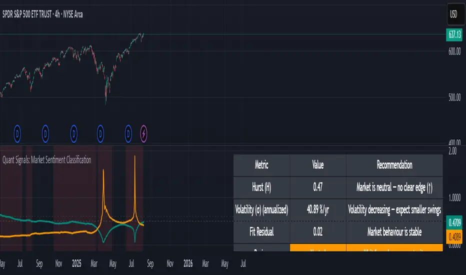
Quant Signals: Market Sentiment Monitor HUDWavelets & Scale Spectrum
This indicator is ideal for traders who adapt their strategy to market conditions — such as swing traders, intraday traders, and system developers.
Trend-followers can use it to confirm trending conditions before entering.
Mean-reversion traders can spot choppy markets where reversals are more likely.
Risk managers can monitor volatility shifts and regime changes to adjust position size or pause trading.
It works best as a market context filter — telling you the “weather” before you decide on the trade.
Wavelets are like tiny “measuring rulers” for price changes. Instead of looking at the whole chart at once, a wavelet looks at differences in price over a specific time scale — for example, 2 bars, 4 bars, 8 bars, and so on.
The scale spectrum is what you get when you measure volatility at several of these scales and then plot them against scale size.
If the spectrum forms a straight line on a log–log chart, it means price changes follow a consistent pattern across time scales (a power-law relationship).
The slope of that line gives the Hurst exponent (H) — telling you whether moves tend to persist (trend) or reverse (mean-revert).
The height of the line gives you the volatility (σ) — the average size of moves.
This approach works like a microscope, revealing whether the market’s behaviour is consistent across short-term and long-term horizons, and when that behaviour changes.
This tool applies a wavelet-based scale-spectrum analysis to price data to estimate three key market state measures inside a rolling window:
Hurst exponent (H) — measures persistence in price moves:
H > ~0.55 → market is trending (moves tend to continue).
H < ~0.45 → market is choppy/mean-reverting (moves tend to reverse).
Values near 0.5 indicate a neutral, random-walk-like regime.
Volatility (σ) — the average size of price swings at your chart’s timeframe, optionally annualized. Rising volatility means larger price moves, falling volatility means smaller moves.
Fit residual — how well the observed multi-scale volatility fits a clean power-law line. Low residual = stable behaviour; high residual = structural change (possible regime shift).
3D Surface Modeling [PhenLabs]📊 3D Surface Modeling
Version: PineScript™ v6
📌 Description
The 3D Surface Modeling indicator revolutionizes technical analysis by generating three-dimensional visualizations of multiple technical indicators across various timeframes. This advanced analytical tool processes and renders complex indicator data through a sophisticated matrix-based calculation system, creating an intuitive 3D surface representation of market dynamics.
The indicator employs array-based computations to simultaneously analyze multiple instances of selected technical indicators, mapping their behavior patterns across different temporal dimensions. This unique approach enables traders to identify complex market patterns and relationships that may be invisible in traditional 2D charts.
🚀 Points of Innovation
Matrix-Based Computation Engine: Processes up to 500 concurrent indicator calculations in real-time
Dynamic 3D Rendering System: Creates depth perception through sophisticated line arrays and color gradients
Multi-Indicator Integration: Seamlessly combines VWAP, Hurst, RSI, Stochastic, CCI, MFI, and Fractal Dimension analyses
Adaptive Scaling Algorithm: Automatically adjusts visualization parameters based on indicator type and market conditions
🔧 Core Components
Indicator Processing Module: Handles real-time calculation of multiple technical indicators using array-based mathematics
3D Visualization Engine: Converts indicator data into three-dimensional surfaces using line arrays and color mapping
Dynamic Scaling System: Implements custom normalization algorithms for different indicator types
Color Gradient Generator: Creates depth perception through programmatic color transitions
🔥 Key Features
Multi-Indicator Support: Comprehensive analysis across seven different technical indicators
Customizable Visualization: User-defined color schemes and line width parameters
Real-time Processing: Continuous calculation and rendering of 3D surfaces
Cross-Timeframe Analysis: Simultaneous visualization of indicator behavior across multiple periods
🎨 Visualization
Surface Plot: Three-dimensional representation using up to 500 lines with dynamic color gradients
Depth Indicators: Color intensity variations showing indicator value magnitude
Pattern Recognition: Visual identification of market structures across multiple timeframes
📖 Usage Guidelines
Indicator Selection
Type: VWAP, Hurst, RSI, Stochastic, CCI, MFI, Fractal Dimension
Default: VWAP
Starting Length: Minimum 5 periods
Default: 10
Step Size: Interval between calculations
Range: 1-10
Visualization Parameters
Color Scheme: Green, Red, Blue options
Line Width: 1-5 pixels
Surface Resolution: Up to 500 lines
✅ Best Use Cases
Multi-timeframe market analysis
Pattern recognition across different technical indicators
Trend strength assessment through 3D visualization
Market behavior study across multiple periods
⚠️ Limitations
High computational resource requirements
Maximum 500 line restriction
Requires substantial historical data
Complex visualization learning curve
🔬 How It Works
1. Data Processing:
Calculates selected indicator values across multiple timeframes
Stores results in multi-dimensional arrays
Applies custom scaling algorithms
2. Visualization Generation:
Creates line arrays for 3D surface representation
Applies color gradients based on value magnitude
Renders real-time updates to surface plot
3. Display Integration:
Synchronizes with chart timeframe
Updates surface plot dynamically
Maintains visual consistency across updates
🌟 Credits:
Inspired by LonesomeTheBlue (modified for multiple indicator types with scaling fixes and additional unique mappings)
💡 Note:
Optimal performance requires sufficient computing resources and historical data. Users should start with default settings and gradually adjust parameters based on their analysis requirements and system capabilities.

Cointegration Buy and Sell Signals [EdgeTerminal]The Cointegration Buy And Sell Signals is a sophisticated technical analysis tool to spot high-probability market turning points — before they fully develop on price charts.
Most reversal indicators rely on raw price action, visual patterns, or basic and common indicator logic — which often suffer in noisy or trending markets. In most cases, they lag behind the actual change in trend and provide useless and late signals.
This indicator is rooted in advanced concepts from statistical arbitrage, mean reversion theory, and quantitative finance, and it packages these ideas in a user-friendly visual format that works on any timeframe and asset class.
It does this by analyzing how the short-term and long-term EMAs behave relative to each other — and uses statistical filters like Z-score, correlation, volatility normalization, and stationarity tests to issue highly selective Buy and Sell signals.
This tool provides statistical confirmation of trend exhaustion, allowing you to trade mean-reverting setups. It fades overextended moves and uses signal stacking to reduce false entries. The entire indicator is based on a very interesting mathematically grounded model which I will get into down below.
Here’s how the indicator works at a high level:
EMAs as Anchors: It starts with two Exponential Moving Averages (EMAs) — one short-term and one long-term — to track market direction.
Statistical Spread (Regression Residuals): It performs a rolling linear regression between the short and long EMA. Instead of using the raw difference (short - long), it calculates the regression residual, which better models their natural relationship.
Normalize the Spread: The spread is divided by historical price volatility (ATR) to make it scale-invariant. This ensures the indicator works on low-priced stocks, high-priced indices, and crypto alike.
Z-Score: It computes a Z-score of the normalized spread to measure how “extreme” the current deviation is from its historical average.
Dynamic Thresholds: Unlike most tools that use fixed thresholds (like Z = ±2), this one calculates dynamic thresholds using historical percentiles (e.g., top 10% and bottom 10%) so that it adapts to the asset's current behavior to reduce false signals based on market’s extreme volatility at a certain time.
Z-Score Momentum: It tracks the direction of the Z-score — if Z is extreme but still moving away from zero, it's too early. It waits for reversion to start (Z momentum flips).
Correlation Check: Uses a rolling Pearson correlation to confirm the two EMAs are still statistically related. If they diverge (low correlation), no signal is shown.
Stationarity Filter (ADF-like): Uses the volatility of the regression residual to determine if the spread is stationary (mean-reverting) — a key concept in cointegration and statistical arbitrage. It’s not possible to build an exact ADF filter in Pine Script so we used the next best thing.
Signal Control: Prevents noisy charts and overtrading by ensuring no back-to-back buy or sell signals. Each signal must alternate and respect a cooldown period so you won’t be overwhelmed and won’t get a messy chart.
Important Notes to Remember:
The whole idea behind this indicator is to try to use some stat arb models to detect shifting patterns faster than they appear on common indicators, so in some cases, some assumptions are made based on historic values.
This means that in some cases, the indicator can “jump” into the conclusion too quickly. Although we try to eliminate this by using stationary filters, correlation checks, and Z-score momentum detection, there is still a chance some signals that are generated can be too early, in the stock market, that's the same as being incorrect. So make sure to use this with other indicators to confirm the movement.
How To Use The Indicator:
You can use the indicator as a standalone reversal system, as a filter for overbought and oversold setups, in combination with other trend indicators and as a part of a signal stack with other common indicators for divergence spotting and fade trades.
The indicator produces simple buy and sell signals when all criteria is met. Based on our own testing, we recommend treating these signals as standalone and independent from each other . Meaning that if you take position after a buy signal, don’t wait for a sell signal to appear to exit the trade and vice versa.
This is why we recommend using this indicator with other advanced or even simple indicators as an early confirmation tool.
The Display Table:
The floating diagnostic table in the top-right corner of the chart is a key part of this indicator. It's a live statistical dashboard that helps you understand why a signal is (or isn’t) being triggered, and whether the market conditions are lining up for a potential reversal.
1. Z-Score
What it shows: The current Z-score value of the volatility-normalized spread between the short EMA and the regression line of the long EMA.
Why it matters: Z-score tells you how statistically extreme the current relationship is. A Z-score of:
0 = perfectly average
> +2 = very overbought
< -2 = very oversold
How to use it: Look for Z-score reaching extreme highs or lows (beyond dynamic thresholds). Watch for it to start reversing direction, especially when paired with green table rows (see below)
2. Z-Score Momentum
What it shows: The rate of change (ROC) of the Z-score:
Zmomentum=Zt − Zt − 1
Why it matters: This tells you if the Z-score is still stretching out (e.g., getting more overbought/oversold), or reverting back toward the mean.
How to use it: A positive Z-momentum after a very low Z-score = potential bullish reversal A negative Z-momentum after a very high Z-score = potential bearish reversal. Avoid signals when momentum is still pushing deeper into extremes
3. Correlation
What it shows: The rolling Pearson correlation coefficient between the short EMA and long EMA.
Why it matters: High correlation (closer to +1) means the EMAs are still statistically connected — a key requirement for cointegration or mean reversion to be valid.
How to use it: Look for correlation > 0.7 for reliable signals. If correlation drops below 0.5, ignore the Z-score — the EMAs aren’t moving together anymore
4. Stationary
What it shows: A simplified "Yes" or "No" answer to the question:
“Is the spread statistically stable (stationary) and mean-reverting right now?”
Why it matters: Mean reversion strategies only work when the spread is stationary — that is, when the distance between EMAs behaves like a rubber band, not a drifting cloud.
How to use it: A "Yes" means the indicator sees a consistent, stable spread — good for trading. "No" means the market is too volatile, disjointed, or chaotic for reliable mean reversion. Wait for this to flip to "Yes" before trusting signals
5. Last Signal
What it shows: The last signal issued by the system — either "Buy", "Sell", or "None"
Why it matters: Helps avoid confusion and repeated entries. Signals only alternate — you won’t get another Buy until a Sell happens, and vice versa.
How to use it: If the last signal was a "Buy", and you’re watching for a Sell, don’t act on more bullish signals. Great for systems where you only want one position open at a time
6. Bars Since Signal
What it shows: How many bars (candles) have passed since the last Buy or Sell signal.
Why it matters: Gives you context for how long the current condition has persisted
How to use it: If it says 1 or 2, a signal just happened — avoid jumping in late. If it’s been 10+ bars, a new opportunity might be brewing soon. You can use this to time exits if you want to fade a recent signal manually
Indicator Settings:
Short EMA: Sets the short-term EMA period. The smaller the number, the more reactive and more signals you get.
Long EMA: Sets the slow EMA period. The larger this number is, the smoother baseline, and more reliable trend bases are generated.
Z-Score Lookback: The period or bars used for mean & std deviation of spread between short and long EMAs. Larger values result in smoother signals with fewer false positives.
Volatility Window: This value normalizes the spread by historical volatility. This allows you to prevent scale distortion, showing you a cleaner and better chart.
Correlation Lookback: How many periods or how far back to test correlation between slow and long EMAs. This filters out false positives when EMAs lose alignment.
Hurst Lookback: The multiplier to approximate stationarity. Lower leads to more sensitivity to regime change, higher produces a more stricter filtering.
Z Threshold Percentile: This value sets how extreme Z-score must be to trigger a signal. For example, 90 equals only top/bottom 10% of extremes, 80 = more frequent.
Min Bars Between Signals: This hard stop prevents back-to-back signals. The idea is to avoid over-trading or whipsaws in volatile markets even when Hurst lookback and volatility window values are not enough to filter signals.
Some More Recommendations:
We recommend trying different EMA pairs (10/50, 21/100, 5/20) for different asset behaviors. You can set percentile to 85 or 80 if you want more frequent but looser signals. You can also use the Z-score reversion monitor for powerful confirmation.

QuantumSync Pulse [ w.aritas ]QuantumSync Pulse (QSP) is an advanced technical indicator crafted for traders seeking a dynamic and adaptable tool to analyze diverse market conditions. By integrating momentum, mean reversion, and regime detection with quantum-inspired calculations and entropy analysis, QSP offers a powerful histogram that reflects trend strength and market uncertainty. With multi-timeframe synchronization, adaptive filtering, and customizable visualization, it’s a versatile addition to any trading strategy.
Key Features
Hybrid Signals: Combines momentum and mean reversion, dynamically weighted by market regime.
Quantum Tunneling: Enhances responsiveness in volatile markets using volatility-adjusted calculations.
3-State Entropy: Assesses market uncertainty across up, down, and neutral states.
Regime Detection: Adapts signal weights with Hurst exponent and volatility ROC.
Multi-Timeframe Alignment: Syncs with higher timeframe trends for context.
Customizable Histogram: Displays trend strength with ADX-based visuals and flexible styling.
How to Use and Interpret
Histogram Interpretation
Positive (Above Zero): Bullish momentum; color intensity shows trend strength.
Negative (Below Zero): Bearish momentum; gradients indicate weakness.
Overlaps: Alignment of final_z (signal) and ohlc4 (price) histograms highlights key price levels or turning points.
Regime Visualization
Green Background: Trending market; prioritize momentum signals.
Red Background: Mean-reverting market; focus on reversion signals.
Blue Background: Neutral state; balance both signal types.
Trading Signals
Buy: Histogram crosses above zero or shows positive divergence between histograms.
Sell: Histogram crosses below zero or exhibits negative divergence.
Confirmation: Match signals with regime background—green for trends, red for ranges.
Customization
Tweak Momentum Length, Entropy Lookback, and Hurst Exponent Lookback for sensitivity.
Adjust color themes and transparency to suit your charts.
Tips for Optimal Use
Timeframes: Use higher timeframes (1h, 4h) for trend context and lower (5m, 15m) for entries.
Pairing: Combine with RSI, MACD, or volume indicators for confirmation.
Backtesting: Test settings on historical data for asset-specific optimization.
Overlaps: Watch for histogram overlaps to identify support, resistance, or reversals.
Simulated Performance
Trending Markets: Histogram stays above/below zero, with overlaps at retracements for entries.
Range-Bound Markets: Oscillates around zero; overlaps signal reversals in red regimes.
Volatile Markets: Quantum tunneling ensures quick reactions, with filters reducing noise.
Elevate your trading with QuantumSync Pulse—a sophisticated tool that adapts to the market’s rhythm and your unique style.

Commitment of Trader %R StrategyThis Pine Script strategy utilizes the Commitment of Traders (COT) data to inform trading decisions based on the Williams %R indicator. The script operates in TradingView and includes various functionalities that allow users to customize their trading parameters.
Here’s a breakdown of its key components:
COT Data Import:
The script imports the COT library from TradingView to access historical COT data related to different trader groups (commercial hedgers, large traders, and small traders).
User Inputs:
COT data selection mode (e.g., Auto, Root, Base currency).
Whether to include futures, options, or both.
The trader group to analyze.
The lookback period for calculating the Williams %R.
Upper and lower thresholds for triggering trades.
An option to enable or disable a Simple Moving Average (SMA) filter.
Williams %R Calculation: The script calculates the Williams %R value, which is a momentum indicator that measures overbought or oversold levels based on the highest and lowest prices over a specified period.
SMA Filter: An optional SMA filter allows users to limit trades to conditions where the price is above or below the SMA, depending on the configuration.
Trade Logic: The strategy enters long positions when the Williams %R value exceeds the upper threshold and exits when the value falls below it. Conversely, it enters short positions when the Williams %R value is below the lower threshold and exits when the value rises above it.
Visual Elements: The script visually indicates the Williams %R values and thresholds on the chart, with the option to plot the SMA if enabled.
Commitment of Traders (COT) Data
The COT report is a weekly publication by the Commodity Futures Trading Commission (CFTC) that provides a breakdown of open interest positions held by different types of traders in the U.S. futures markets. It is widely used by traders and analysts to gauge market sentiment and potential price movements.
Data Collection: The COT data is collected from futures commission merchants and is published every Friday, reflecting positions as of the previous Tuesday. The report categorizes traders into three main groups:
Commercial Traders: These are typically hedgers (like producers and processors) who use futures to mitigate risk.
Non-Commercial Traders: Often referred to as speculators, these traders do not have a commercial interest in the underlying commodity but seek to profit from price changes.
Non-reportable Positions: Small traders who do not meet the reporting threshold set by the CFTC.
Interpretation:
Market Sentiment: By analyzing the positions of different trader groups, market participants can gauge sentiment. For instance, if commercial traders are heavily short, it may suggest they expect prices to decline.
Extreme Positions: Some traders look for extreme positions among non-commercial traders as potential reversal signals. For example, if speculators are overwhelmingly long, it might indicate an overbought condition.
Statistical Insights: COT data is often used in conjunction with technical analysis to inform trading decisions. Studies have shown that analyzing COT data can provide valuable insights into future price movements (Lund, 2018; Hurst et al., 2017).
Scientific References
Lund, J. (2018). Understanding the COT Report: An Analysis of Speculative Trading Strategies.
Journal of Derivatives and Hedge Funds, 24(1), 41-52. DOI:10.1057/s41260-018-00107-3
Hurst, B., O'Neill, R., & Roulston, M. (2017). The Impact of COT Reports on Futures Market Prices: An Empirical Analysis. Journal of Futures Markets, 37(8), 763-785.
DOI:10.1002/fut.21849
Commodity Futures Trading Commission (CFTC). (2024). Commitment of Traders. Retrieved from CFTC Official Website.

Intramarket Difference Index StrategyHi Traders !!
The IDI Strategy:
In layman’s terms this strategy compares two indicators across markets and exploits their differences.
note: it is best the two markets are correlated as then we know we are trading a short to long term deviation from both markets' general trend with the assumption both markets will trend again sometime in the future thereby exhausting our trading opportunity.
📍 Import Notes:
This Strategy calculates trade position size independently (i.e. risk per trade is controlled in the user inputs tab), this means that the ‘Order size’ input in the ‘Properties’ tab will have no effect on the strategy. Why ? because this allows us to define custom position size algorithms which we can use to improve our risk management and equity growth over time. Here we have the option to have fixed quantity or fixed percentage of equity ATR (Average True Range) based stops in addition to the turtle trading position size algorithm.
‘Pyramiding’ does not work for this strategy’, similar to the order size input togeling this input will have no effect on the strategy as the strategy explicitly defines the maximum order size to be 1.
This strategy is not perfect, and as of writing of this post I have not traded this algo.
Always take your time to backtests and debug the strategy.
🔷 The IDI Strategy:
By default this strategy pulls data from your current TV chart and then compares it to the base market, be default BINANCE:BTCUSD . The strategy pulls SMA and RSI data from either market (we call this the difference data), standardizes the data (solving the different unit problem across markets) such that it is comparable and then differentiates the data, calling the result of this transformation and difference the Intramarket Difference (ID). The formula for the the ID is
ID = market1_diff_data - market2_diff_data (1)
Where
market(i)_diff_data = diff_data / ATR(j)_market(i)^0.5,
where i = {1, 2} and j = the natural numbers excluding 0
Formula (1) interpretation is the following
When ID > 0: this means the current market outperforms the base market
When ID = 0: Markets are at long run equilibrium
When ID < 0: this means the current market underperforms the base market
To form the strategy we define one of two strategy type’s which are Trend and Mean Revesion respectively.
🔸 Trend Case:
Given the ‘‘Strategy Type’’ is equal to TREND we define a threshold for which if the ID crosses over we go long and if the ID crosses under the negative of the threshold we go short.
The motivating idea is that the ID is an indicator of the two symbols being out of sync, and given we know volatility clustering, momentum and mean reversion of anomalies to be a stylised fact of financial data we can construct a trading premise. Let's first talk more about this premise.
For some markets (cryptocurrency markets - synthetic symbols in TV) the stylised fact of momentum is true, this means that higher momentum is followed by higher momentum, and given we know momentum to be a vector quantity (with magnitude and direction) this momentum can be both positive and negative i.e. when the ID crosses above some threshold we make an assumption it will continue in that direction for some time before executing back to its long run equilibrium of 0 which is a reasonable assumption to make if the market are correlated. For example for the BTCUSD - ETHUSD pair, if the ID > +threshold (inputs for MA and RSI based ID thresholds are found under the ‘‘INTRAMARKET DIFFERENCE INDEX’’ group’), ETHUSD outperforms BTCUSD, we assume the momentum to continue so we go long ETHUSD.
In the standard case we would exit the market when the IDI returns to its long run equilibrium of 0 (for the positive case the ID may return to 0 because ETH’s difference data may have decreased or BTC’s difference data may have increased). However in this strategy we will not define this as our exit condition, why ?
This is because we want to ‘‘let our winners run’’, to achieve this we define a trailing Donchian Channel stop loss (along with a fixed ATR based stop as our volatility proxy). If we were too use the 0 exit the strategy may print a buy signal (ID > +threshold in the simple case, market regimes may be used), return to 0 and then print another buy signal, and this process can loop may times, this high trade frequency means we fail capture the entire market move lowering our profit, furthermore on lower time frames this high trade frequencies mean we pay more transaction costs (due to price slippage, commission and big-ask spread) which means less profit.
By capturing the sum of many momentum moves we are essentially following the trend hence the trend following strategy type.
Here we also print the IDI (with default strategy settings with the MA difference type), we can see that by letting our winners run we may catch many valid momentum moves, that results in a larger final pnl that if we would otherwise exit based on the equilibrium condition(Valid trades are denoted by solid green and red arrows respectively and all other valid trades which occur within the original signal are light green and red small arrows).
another example...
Note: if you would like to plot the IDI separately copy and paste the following code in a new Pine Script indicator template.
indicator("IDI")
// INTRAMARKET INDEX
var string g_idi = "intramarket diffirence index"
ui_index_1 = input.symbol("BINANCE:BTCUSD", title = "Base market", group = g_idi)
// ui_index_2 = input.symbol("BINANCE:ETHUSD", title = "Quote Market", group = g_idi)
type = input.string("MA", title = "Differrencing Series", options = , group = g_idi)
ui_ma_lkb = input.int(24, title = "lookback of ma and volatility scaling constant", group = g_idi)
ui_rsi_lkb = input.int(14, title = "Lookback of RSI", group = g_idi)
ui_atr_lkb = input.int(300, title = "ATR lookback - Normalising value", group = g_idi)
ui_ma_threshold = input.float(5, title = "Threshold of Upward/Downward Trend (MA)", group = g_idi)
ui_rsi_threshold = input.float(20, title = "Threshold of Upward/Downward Trend (RSI)", group = g_idi)
//>>+----------------------------------------------------------------+}
// CUSTOM FUNCTIONS |
//<<+----------------------------------------------------------------+{
// construct UDT (User defined type) containing the IDI (Intramarket Difference Index) source values
// UDT will hold many variables / functions grouped under the UDT
type functions
float Close // close price
float ma // ma of symbol
float rsi // rsi of the asset
float atr // atr of the asset
// the security data
getUDTdata(symbol, malookback, rsilookback, atrlookback) =>
indexHighTF = barstate.isrealtime ? 1 : 0
= request.security(symbol, timeframe = timeframe.period,
expression = [close , // Instentiate UDT variables
ta.sma(close, malookback) ,
ta.rsi(close, rsilookback) ,
ta.atr(atrlookback) ])
data = functions.new(close_, ma_, rsi_, atr_)
data
// Intramerket Difference Index
idi(type, symbol1, malookback, rsilookback, atrlookback, mathreshold, rsithreshold) =>
threshold = float(na)
index1 = getUDTdata(symbol1, malookback, rsilookback, atrlookback)
index2 = getUDTdata(syminfo.tickerid, malookback, rsilookback, atrlookback)
// declare difference variables for both base and quote symbols, conditional on which difference type is selected
var diffindex1 = 0.0, var diffindex2 = 0.0,
// declare Intramarket Difference Index based on series type, note
// if > 0, index 2 outpreforms index 1, buy index 2 (momentum based) until equalibrium
// if < 0, index 2 underpreforms index 1, sell index 1 (momentum based) until equalibrium
// for idi to be valid both series must be stationary and normalised so both series hae he same scale
intramarket_difference = 0.0
if type == "MA"
threshold := mathreshold
diffindex1 := (index1.Close - index1.ma) / math.pow(index1.atr*malookback, 0.5)
diffindex2 := (index2.Close - index2.ma) / math.pow(index2.atr*malookback, 0.5)
intramarket_difference := diffindex2 - diffindex1
else if type == "RSI"
threshold := rsilookback
diffindex1 := index1.rsi
diffindex2 := index2.rsi
intramarket_difference := diffindex2 - diffindex1
//>>+----------------------------------------------------------------+}
// STRATEGY FUNCTIONS CALLS |
//<<+----------------------------------------------------------------+{
// plot the intramarket difference
= idi(type,
ui_index_1,
ui_ma_lkb,
ui_rsi_lkb,
ui_atr_lkb,
ui_ma_threshold,
ui_rsi_threshold)
//>>+----------------------------------------------------------------+}
plot(intramarket_difference, color = color.orange)
hline(type == "MA" ? ui_ma_threshold : ui_rsi_threshold, color = color.green)
hline(type == "MA" ? -ui_ma_threshold : -ui_rsi_threshold, color = color.red)
hline(0)
Note it is possible that after printing a buy the strategy then prints many sell signals before returning to a buy, which again has the same implication (less profit. Potentially because we exit early only for price to continue upwards hence missing the larger "trend"). The image below showcases this cenario and again, by allowing our winner to run we may capture more profit (theoretically).
This should be clear...
🔸 Mean Reversion Case:
We stated prior that mean reversion of anomalies is an standerdies fact of financial data, how can we exploit this ?
We exploit this by normalizing the ID by applying the Ehlers fisher transformation. The transformed data is then assumed to be approximately normally distributed. To form the strategy we employ the same logic as for the z score, if the FT normalized ID > 2.5 (< -2.5) we buy (short). Our exit conditions remain unchanged (fixed ATR stop and trailing Donchian Trailing stop)
🔷 Position Sizing:
If ‘‘Fixed Risk From Initial Balance’’ is toggled true this means we risk a fixed percentage of our initial balance, if false we risk a fixed percentage of our equity (current balance).
Note we also employ a volatility adjusted position sizing formula, the turtle training method which is defined as follows.
Turtle position size = (1/ r * ATR * DV) * C
Where,
r = risk factor coefficient (default is 20)
ATR(j) = risk proxy, over j times steps
DV = Dollar Volatility, where DV = (1/Asset Price) * Capital at Risk
🔷 Risk Management:
Correct money management means we can limit risk and increase reward (theoretically). Here we employ
Max loss and gain per day
Max loss per trade
Max number of consecutive losing trades until trade skip
To read more see the tooltips (info circle).
🔷 Take Profit:
By defualt the script uses a Donchain Channel as a trailing stop and take profit, In addition to this the script defines a fixed ATR stop losses (by defualt, this covers cases where the DC range may be to wide making a fixed ATR stop usefull), ATR take profits however are defined but optional.
ATR SL and TP defined for all trades
🔷 Hurst Regime (Regime Filter):
The Hurst Exponent (H) aims to segment the market into three different states, Trending (H > 0.5), Random Geometric Brownian Motion (H = 0.5) and Mean Reverting / Contrarian (H < 0.5). In my interpretation this can be used as a trend filter that eliminates market noise.
We utilize the trending and mean reverting based states, as extra conditions required for valid trades for both strategy types respectively, in the process increasing our trade entry quality.
🔷 Example model Architecture:
Here is an example of one configuration of this strategy, combining all aspects discussed in this post.
Future Updates
- Automation integration (next update)
Musashi_Fractal_Dimension === Musashi-Fractal-Dimension ===
This tool is part of my research on the fractal nature of the markets and understanding the relation between fractal dimension and chaos theory.
To take full advantage of this indicator, you need to incorporate some principles and concepts:
- Traditional Technical Analysis is linear and Euclidean, which makes very difficult its modeling.
- Linear techniques cannot quantify non-linear behavior
- Is it possible to measure accurately a wave or the surface of a mountain with a simple ruler?
- Fractals quantify what Euclidean Geometry can’t, they measure chaos, as they identify order in apparent randomness.
- Remember: Chaos is order disguised as randomness.
- Chaos is the study of unstable aperiodic behavior in deterministic non-linear dynamic systems
- Order and randomness can coexist, allowing predictability.
- There is a reason why Fractal Dimension was invented, we had no way of measuring fractal-based structures.
- Benoit Mandelbrot used to explain it by asking: How do we measure the coast of Great Britain?
- An easy way of getting the need of a dimension in between is looking at the Koch snowflake.
- Market prices tend to seek natural levels of ranges of balance. These levels can be described as attractors and are determinant.
Fractal Dimension Index ('FDI')
Determines the persistence or anti-persistence of a market.
- A persistent market follows a market trend. An anti-persistent market results in substantial volatility around the trend (with a low r2), and is more vulnerable to price reversals
- An easy way to see this is to think that fractal dimension measures what is in between mainstream dimensions. These are:
- One dimension: a line
- Two dimensions: a square
- Three dimensions: a cube.
--> This will hint you that at certain moment, if the market has a Fractal Dimension of 1.25 (which is low), the market is behaving more “line-like”, while if the market has a high Fractal Dimension, it could be interpreted as “square-like”.
- 'FDI' is trend agnostic, which means that doesn't consider trend. This makes it super useful as gives you clean information about the market without trying to include trend stuff.
Question: If we have a game where you must choose between two options.
1. a horizontal line
2. a vertical line.
Each iteration a Horizontal Line or a Square will appear as continuation of a figure. If it that iteration shows a square and you bet vertical you win, same as if it is horizontal and it is a line.
- Wouldn’t be useful to know that Fractal dimension is 1.8? This will hint square. In the markets you can use 'FD' to filter mean-reversal signals like Bollinger bands, stochastics, Regular RSI divergences, etc.
- Wouldn’t be useful to know that Fractal dimension is 1.2? This will hint Line. In the markets you can use 'FD' to confirm trend following strategies like Moving averages, MACD, Hidden RSI divergences.
Calculation method:
Fractal dimension is obtained from the ‘hurst exponent’.
'FDI' = 2 - 'Hurst Exponent'
Musashi version of the Classic 'OG' Fractal Dimension Index ('FDI')
- By default, you get 3 fast 'FDI's (11,12,13) + 1 Slow 'FDI' (21), their interaction gives useful information.
- Fast 'FDI' cross will give you gray or red dots while Slow 'FDI' cross with the slowest of the fast 'FDI's will give white and orange dots. This are great to early spot trend beginnings or trend ends.
- A baseline (purple) is also provided, this is calculated using a 21 period Bollinger bands with 1.618 'SD', once calculated, you just take midpoint, this is the 'TDI's (Traders Dynamic Index) way. The indicator will print purple dots when Slow 'FDI' and baseline crosses, I see them as Short-Term cycle changes.
- Negative slope 'FDI' means trending asset.
- Positive most of the times hints correction, but if it got overextended it might hint a rocket-shot.
TDI Ranges:
- 'FDI' between 1.0≤ 'FDI' ≤1.4 will confirm trend following continuation signals.
- 'FDI' between 1.6≥ 'FDI' ≥2.0 will confirm reversal signals.
- 'FDI' == 1.5 hints a random unpredictable market.
Fractal Attractors
- As you must know, fractals tend orbit certain spots, this are named Attractors, this happens with any fractal behavior. The market of course also shows them, in form of Support & Resistance, Supply Demand, etc. It’s obvious they are there, but now we understand that they’re not linear, as the market is fractal, so simple trendline might not be the best tool to model this.
- I’ve noticed that when the Musashi version of the 'FDI' indicator start making a cluster of multicolor dots, this end up being an attractor, I tend to draw a rectangle as that area as price tend to come back (I still researching here).
Extra useful stuff
- Momentum / speed: Included by checking RSI Study in the indicator properties. This will add two RSI’s (9 and a 7 periods) plus a baseline calculated same way as explained for 'FDI'. This gives accurate short-term trends. It also includes RSI divergences (regular and hidden), deactivate with a simple check in the RSI section of the properties.
- BBWP (Bollinger Bands with Percentile): Efficient way of visualizing volatility as the percentile of Bollinger bands expansion. This line varies color from Iced blue when low volatility and magma red when high. By default, comes with the High vols deactivated for better view of 'FDI' and RSI while all studies are included. DDWP is trend agnostic, just like 'FDI', which make it very clean at providing information.
- Ultra Slow 'FDI': I noticed that while using BBWP and RSI, the indicator gets overcrowded, so there is the possibility of adding only one 'FDI' + its baseline.
Final Note: I’ve shown you few ways of using this indicator, please backtest before using in real trading. As you know trading is more about risk and trade management than the strategy used. This still a work in progress, I really hope you find value out of it. I use it combination with a tool named “Musashi_Katana” (also found in TradingView).
Best!
Musashi

MA ClustersBackground :
This study allows to define ranges for contraction and expansion of a defined set of MA to analyse the the momentum at those specific situations.
In general all functions used are very basic but allows the user to set alerts when a cluster of MA enters a defined range within or outside the MAX and MIN of a selected MA cluster. The predefined length of the EMAs were put together by HurstHorns within a trading learning discord group and are designed for 1M timeframe to read the momentum for scalping entries - Thanks again for sharing.
Functions :
currently the following MA are available:
- ema
- sma
- smma
- wma
- vwma
- vma
the variable moving average is based on the calculation from lazybear.
- RSI Stoch Filter
- Wavetrend OB/OS filter
Currently only alerts for contraction are enabled to not overload the study but in case expansion would be from interest this can be added quickly.
Outlook:
Additional filters were added to see if they can add value in. the decision making or by simply filtering out noise. This is still quite experimental. Please share any useful observation I should add as additional filter option to find good setups. in relation to contractions or expansions.
Next version will get Bollinger bands for 1 selectable MA from the list for additional study options.
In case you are interested in more options such as more MA types or vwap.. just let me know. for VMA I need to do more research to add useful function for laddering or things like that.
In general The script itself can be easily extended by additional functions. As this is one of my first scripts the code itself might not be optimal or there are more elegant ways to come to the same goal. However please use for study purposes only and report bugs or enhancement requests.
good luck and happy trading!

Harmonic Sine Waves model plot Hey,
Here is another tool that I created. I could not find anything similar.
This script is creating a sine wave, based on the given length, amplitude, horizontal vertical offset.
After this it plots also nearest harmonics to the base sine wave and draws it on the chart.
At the last step it sums up the value for base sine wave with its harmonics.
This is a great way to experience how 4 basic sine waves, when summed up, are creating more complex chart.
This shows that the 'chaotic' chart can be built on just a few most important factors.
You do not have to "know every single fact" about the asset to make a proper forecast.
You just need those most important.
It is crucial though, to offset the chart in a correct way, so it is in phase with the asset that we work on.

Advanced Bitcoin Cycle Detector with Projections & Hursttest script created with openrouter adn google gemmi 3

Dimensional Resonance ProtocolDimensional Resonance Protocol
🌀 CORE INNOVATION: PHASE SPACE RECONSTRUCTION & EMERGENCE DETECTION
The Dimensional Resonance Protocol represents a paradigm shift from traditional technical analysis to complexity science. Rather than measuring price levels or indicator crossovers, DRP reconstructs the hidden attractor governing market dynamics using Takens' embedding theorem, then detects emergence —the rare moments when multiple dimensions of market behavior spontaneously synchronize into coherent, predictable states.
The Complexity Hypothesis:
Markets are not simple oscillators or random walks—they are complex adaptive systems existing in high-dimensional phase space. Traditional indicators see only shadows (one-dimensional projections) of this higher-dimensional reality. DRP reconstructs the full phase space using time-delay embedding, revealing the true structure of market dynamics.
Takens' Embedding Theorem (1981):
A profound mathematical result from dynamical systems theory: Given a time series from a complex system, we can reconstruct its full phase space by creating delayed copies of the observation.
Mathematical Foundation:
From single observable x(t), create embedding vectors:
X(t) =
Where:
• d = Embedding dimension (default 5)
• τ = Time delay (default 3 bars)
• x(t) = Price or return at time t
Key Insight: If d ≥ 2D+1 (where D is the true attractor dimension), this embedding is topologically equivalent to the actual system dynamics. We've reconstructed the hidden attractor from a single price series.
Why This Matters:
Markets appear random in one dimension (price chart). But in reconstructed phase space, structure emerges—attractors, limit cycles, strange attractors. When we identify these structures, we can detect:
• Stable regions : Predictable behavior (trade opportunities)
• Chaotic regions : Unpredictable behavior (avoid trading)
• Critical transitions : Phase changes between regimes
Phase Space Magnitude Calculation:
phase_magnitude = sqrt(Σ ² for i = 0 to d-1)
This measures the "energy" or "momentum" of the market trajectory through phase space. High magnitude = strong directional move. Low magnitude = consolidation.
📊 RECURRENCE QUANTIFICATION ANALYSIS (RQA)
Once phase space is reconstructed, we analyze its recurrence structure —when does the system return near previous states?
Recurrence Plot Foundation:
A recurrence occurs when two phase space points are closer than threshold ε:
R(i,j) = 1 if ||X(i) - X(j)|| < ε, else 0
This creates a binary matrix showing when the system revisits similar states.
Key RQA Metrics:
1. Recurrence Rate (RR):
RR = (Number of recurrent points) / (Total possible pairs)
• RR near 0: System never repeats (highly stochastic)
• RR = 0.1-0.3: Moderate recurrence (tradeable patterns)
• RR > 0.5: System stuck in attractor (ranging market)
• RR near 1: System frozen (no dynamics)
Interpretation: Moderate recurrence is optimal —patterns exist but market isn't stuck.
2. Determinism (DET):
Measures what fraction of recurrences form diagonal structures in the recurrence plot. Diagonals indicate deterministic evolution (trajectory follows predictable paths).
DET = (Recurrence points on diagonals) / (Total recurrence points)
• DET < 0.3: Random dynamics
• DET = 0.3-0.7: Moderate determinism (patterns with noise)
• DET > 0.7: Strong determinism (technical patterns reliable)
Trading Implication: Signals are prioritized when DET > 0.3 (deterministic state) and RR is moderate (not stuck).
Threshold Selection (ε):
Default ε = 0.10 × std_dev means two states are "recurrent" if within 10% of a standard deviation. This is tight enough to require genuine similarity but loose enough to find patterns.
🔬 PERMUTATION ENTROPY: COMPLEXITY MEASUREMENT
Permutation entropy measures the complexity of a time series by analyzing the distribution of ordinal patterns.
Algorithm (Bandt & Pompe, 2002):
1. Take overlapping windows of length n (default n=4)
2. For each window, record the rank order pattern
Example: → pattern (ranks from lowest to highest)
3. Count frequency of each possible pattern
4. Calculate Shannon entropy of pattern distribution
Mathematical Formula:
H_perm = -Σ p(π) · ln(p(π))
Where π ranges over all n! possible permutations, p(π) is the probability of pattern π.
Normalized to :
H_norm = H_perm / ln(n!)
Interpretation:
• H < 0.3 : Very ordered, crystalline structure (strong trending)
• H = 0.3-0.5 : Ordered regime (tradeable with patterns)
• H = 0.5-0.7 : Moderate complexity (mixed conditions)
• H = 0.7-0.85 : Complex dynamics (challenging to trade)
• H > 0.85 : Maximum entropy (nearly random, avoid)
Entropy Regime Classification:
DRP classifies markets into five entropy regimes:
• CRYSTALLINE (H < 0.3): Maximum order, persistent trends
• ORDERED (H < 0.5): Clear patterns, momentum strategies work
• MODERATE (H < 0.7): Mixed dynamics, adaptive required
• COMPLEX (H < 0.85): High entropy, mean reversion better
• CHAOTIC (H ≥ 0.85): Near-random, minimize trading
Why Permutation Entropy?
Unlike traditional entropy methods requiring binning continuous data (losing information), permutation entropy:
• Works directly on time series
• Robust to monotonic transformations
• Computationally efficient
• Captures temporal structure, not just distribution
• Immune to outliers (uses ranks, not values)
⚡ LYAPUNOV EXPONENT: CHAOS vs STABILITY
The Lyapunov exponent λ measures sensitivity to initial conditions —the hallmark of chaos.
Physical Meaning:
Two trajectories starting infinitely close will diverge at exponential rate e^(λt):
Distance(t) ≈ Distance(0) × e^(λt)
Interpretation:
• λ > 0 : Positive Lyapunov exponent = CHAOS
- Small errors grow exponentially
- Long-term prediction impossible
- System is sensitive, unpredictable
- AVOID TRADING
• λ ≈ 0 : Near-zero = CRITICAL STATE
- Edge of chaos
- Transition zone between order and disorder
- Moderate predictability
- PROCEED WITH CAUTION
• λ < 0 : Negative Lyapunov exponent = STABLE
- Small errors decay
- Trajectories converge
- System is predictable
- OPTIMAL FOR TRADING
Estimation Method:
DRP estimates λ by tracking how quickly nearby states diverge over a rolling window (default 20 bars):
For each bar i in window:
δ₀ = |x - x | (initial separation)
δ₁ = |x - x | (previous separation)
if δ₁ > 0:
ratio = δ₀ / δ₁
log_ratios += ln(ratio)
λ ≈ average(log_ratios)
Stability Classification:
• STABLE : λ < 0 (negative growth rate)
• CRITICAL : |λ| < 0.1 (near neutral)
• CHAOTIC : λ > 0.2 (strong positive growth)
Signal Filtering:
By default, NEXUS requires λ < 0 (stable regime) for signal confirmation. This filters out trades during chaotic periods when technical patterns break down.
📐 HIGUCHI FRACTAL DIMENSION
Fractal dimension measures self-similarity and complexity of the price trajectory.
Theoretical Background:
A curve's fractal dimension D ranges from 1 (smooth line) to 2 (space-filling curve):
• D ≈ 1.0 : Smooth, persistent trending
• D ≈ 1.5 : Random walk (Brownian motion)
• D ≈ 2.0 : Highly irregular, space-filling
Higuchi Method (1988):
For a time series of length N, construct k different curves by taking every k-th point:
L(k) = (1/k) × Σ|x - x | × (N-1)/(⌊(N-m)/k⌋ × k)
For different values of k (1 to k_max), calculate L(k). The fractal dimension is the slope of log(L(k)) vs log(1/k):
D = slope of log(L) vs log(1/k)
Market Interpretation:
• D < 1.35 : Strong trending, persistent (Hurst > 0.5)
- TRENDING regime
- Momentum strategies favored
- Breakouts likely to continue
• D = 1.35-1.45 : Moderate persistence
- PERSISTENT regime
- Trend-following with caution
- Patterns have meaning
• D = 1.45-1.55 : Random walk territory
- RANDOM regime
- Efficiency hypothesis holds
- Technical analysis least reliable
• D = 1.55-1.65 : Anti-persistent (mean-reverting)
- ANTI-PERSISTENT regime
- Oscillator strategies work
- Overbought/oversold meaningful
• D > 1.65 : Highly complex, choppy
- COMPLEX regime
- Avoid directional bets
- Wait for regime change
Signal Filtering:
Resonance signals (secondary signal type) require D < 1.5, indicating trending or persistent dynamics where momentum has meaning.
🔗 TRANSFER ENTROPY: CAUSAL INFORMATION FLOW
Transfer entropy measures directed causal influence between time series—not just correlation, but actual information transfer.
Schreiber's Definition (2000):
Transfer entropy from X to Y measures how much knowing X's past reduces uncertainty about Y's future:
TE(X→Y) = H(Y_future | Y_past) - H(Y_future | Y_past, X_past)
Where H is Shannon entropy.
Key Properties:
1. Directional : TE(X→Y) ≠ TE(Y→X) in general
2. Non-linear : Detects complex causal relationships
3. Model-free : No assumptions about functional form
4. Lag-independent : Captures delayed causal effects
Three Causal Flows Measured:
1. Volume → Price (TE_V→P):
Measures how much volume patterns predict price changes.
• TE > 0 : Volume provides predictive information about price
- Institutional participation driving moves
- Volume confirms direction
- High reliability
• TE ≈ 0 : No causal flow (weak volume/price relationship)
- Volume uninformative
- Caution on signals
• TE < 0 (rare): Suggests price leading volume
- Potentially manipulated or thin market
2. Volatility → Momentum (TE_σ→M):
Does volatility expansion predict momentum changes?
• Positive TE : Volatility precedes momentum shifts
- Breakout dynamics
- Regime transitions
3. Structure → Price (TE_S→P):
Do support/resistance patterns causally influence price?
• Positive TE : Structural levels have causal impact
- Technical levels matter
- Market respects structure
Net Causal Flow:
Net_Flow = TE_V→P + 0.5·TE_σ→M + TE_S→P
• Net > +0.1 : Bullish causal structure
• Net < -0.1 : Bearish causal structure
• |Net| < 0.1 : Neutral/unclear causation
Causal Gate:
For signal confirmation, NEXUS requires:
• Buy signals : TE_V→P > 0 AND Net_Flow > 0.05
• Sell signals : TE_V→P > 0 AND Net_Flow < -0.05
This ensures volume is actually driving price (causal support exists), not just correlated noise.
Implementation Note:
Computing true transfer entropy requires discretizing continuous data into bins (default 6 bins) and estimating joint probability distributions. NEXUS uses a hybrid approach combining TE theory with autocorrelation structure and lagged cross-correlation to approximate information transfer in computationally efficient manner.
🌊 HILBERT PHASE COHERENCE
Phase coherence measures synchronization across market dimensions using Hilbert transform analysis.
Hilbert Transform Theory:
For a signal x(t), the Hilbert transform H (t) creates an analytic signal:
z(t) = x(t) + i·H (t) = A(t)·e^(iφ(t))
Where:
• A(t) = Instantaneous amplitude
• φ(t) = Instantaneous phase
Instantaneous Phase:
φ(t) = arctan(H (t) / x(t))
The phase represents where the signal is in its natural cycle—analogous to position on a unit circle.
Four Dimensions Analyzed:
1. Momentum Phase : Phase of price rate-of-change
2. Volume Phase : Phase of volume intensity
3. Volatility Phase : Phase of ATR cycles
4. Structure Phase : Phase of position within range
Phase Locking Value (PLV):
For two signals with phases φ₁(t) and φ₂(t), PLV measures phase synchronization:
PLV = |⟨e^(i(φ₁(t) - φ₂(t)))⟩|
Where ⟨·⟩ is time average over window.
Interpretation:
• PLV = 0 : Completely random phase relationship (no synchronization)
• PLV = 0.5 : Moderate phase locking
• PLV = 1 : Perfect synchronization (phases locked)
Pairwise PLV Calculations:
• PLV_momentum-volume : Are momentum and volume cycles synchronized?
• PLV_momentum-structure : Are momentum cycles aligned with structure?
• PLV_volume-structure : Are volume and structural patterns in phase?
Overall Phase Coherence:
Coherence = (PLV_mom-vol + PLV_mom-struct + PLV_vol-struct) / 3
Signal Confirmation:
Emergence signals require coherence ≥ threshold (default 0.70):
• Below 0.70: Dimensions not synchronized, no coherent market state
• Above 0.70: Dimensions in phase, coherent behavior emerging
Coherence Direction:
The summed phase angles indicate whether synchronized dimensions point bullish or bearish:
Direction = sin(φ_momentum) + 0.5·sin(φ_volume) + 0.5·sin(φ_structure)
• Direction > 0 : Phases pointing upward (bullish synchronization)
• Direction < 0 : Phases pointing downward (bearish synchronization)
🌀 EMERGENCE SCORE: MULTI-DIMENSIONAL ALIGNMENT
The emergence score aggregates all complexity metrics into a single 0-1 value representing market coherence.
Eight Components with Weights:
1. Phase Coherence (20%):
Direct contribution: coherence × 0.20
Measures dimensional synchronization.
2. Entropy Regime (15%):
Contribution: (0.6 - H_perm) / 0.6 × 0.15 if H < 0.6, else 0
Rewards low entropy (ordered, predictable states).
3. Lyapunov Stability (12%):
• λ < 0 (stable): +0.12
• |λ| < 0.1 (critical): +0.08
• λ > 0.2 (chaotic): +0.0
Requires stable, predictable dynamics.
4. Fractal Dimension Trending (12%):
Contribution: (1.45 - D) / 0.45 × 0.12 if D < 1.45, else 0
Rewards trending fractal structure (D < 1.45).
5. Dimensional Resonance (12%):
Contribution: |dimensional_resonance| × 0.12
Measures alignment across momentum, volume, structure, volatility dimensions.
6. Causal Flow Strength (9%):
Contribution: |net_causal_flow| × 0.09
Rewards strong causal relationships.
7. Phase Space Embedding (10%):
Contribution: min(|phase_magnitude_norm|, 3.0) / 3.0 × 0.10 if |magnitude| > 1.0
Rewards strong trajectory in reconstructed phase space.
8. Recurrence Quality (10%):
Contribution: determinism × 0.10 if DET > 0.3 AND 0.1 < RR < 0.8
Rewards deterministic patterns with moderate recurrence.
Total Emergence Score:
E = Σ(components) ∈
Capped at 1.0 maximum.
Emergence Direction:
Separate calculation determining bullish vs bearish:
• Dimensional resonance sign
• Net causal flow sign
• Phase magnitude correlation with momentum
Signal Threshold:
Default emergence_threshold = 0.75 means 75% of maximum possible emergence score required to trigger signals.
Why Emergence Matters:
Traditional indicators measure single dimensions. Emergence detects self-organization —when multiple independent dimensions spontaneously align. This is the market equivalent of a phase transition in physics, where microscopic chaos gives way to macroscopic order.
These are the highest-probability trade opportunities because the entire system is resonating in the same direction.
🎯 SIGNAL GENERATION: EMERGENCE vs RESONANCE
DRP generates two tiers of signals with different requirements:
TIER 1: EMERGENCE SIGNALS (Primary)
Requirements:
1. Emergence score ≥ threshold (default 0.75)
2. Phase coherence ≥ threshold (default 0.70)
3. Emergence direction > 0.2 (bullish) or < -0.2 (bearish)
4. Causal gate passed (if enabled): TE_V→P > 0 and net_flow confirms direction
5. Stability zone (if enabled): λ < 0 or |λ| < 0.1
6. Price confirmation: Close > open (bulls) or close < open (bears)
7. Cooldown satisfied: bars_since_signal ≥ cooldown_period
EMERGENCE BUY:
• All above conditions met with bullish direction
• Market has achieved coherent bullish state
• Multiple dimensions synchronized upward
EMERGENCE SELL:
• All above conditions met with bearish direction
• Market has achieved coherent bearish state
• Multiple dimensions synchronized downward
Premium Emergence:
When signal_quality (emergence_score × phase_coherence) > 0.7:
• Displayed as ★ star symbol
• Highest conviction trades
• Maximum dimensional alignment
Standard Emergence:
When signal_quality 0.5-0.7:
• Displayed as ◆ diamond symbol
• Strong signals but not perfect alignment
TIER 2: RESONANCE SIGNALS (Secondary)
Requirements:
1. Dimensional resonance > +0.6 (bullish) or < -0.6 (bearish)
2. Fractal dimension < 1.5 (trending/persistent regime)
3. Price confirmation matches direction
4. NOT in chaotic regime (λ < 0.2)
5. Cooldown satisfied
6. NO emergence signal firing (resonance is fallback)
RESONANCE BUY:
• Dimensional alignment without full emergence
• Trending fractal structure
• Moderate conviction
RESONANCE SELL:
• Dimensional alignment without full emergence
• Bearish resonance with trending structure
• Moderate conviction
Displayed as small ▲/▼ triangles with transparency.
Signal Hierarchy:
IF emergence conditions met:
Fire EMERGENCE signal (★ or ◆)
ELSE IF resonance conditions met:
Fire RESONANCE signal (▲ or ▼)
ELSE:
No signal
Cooldown System:
After any signal fires, cooldown_period (default 5 bars) must elapse before next signal. This prevents signal clustering during persistent conditions.
Cooldown tracks using bar_index:
bars_since_signal = current_bar_index - last_signal_bar_index
cooldown_ok = bars_since_signal >= cooldown_period
🎨 VISUAL SYSTEM: MULTI-LAYER COMPLEXITY
DRP provides rich visual feedback across four distinct layers:
LAYER 1: COHERENCE FIELD (Background)
Colored background intensity based on phase coherence:
• No background : Coherence < 0.5 (incoherent state)
• Faint glow : Coherence 0.5-0.7 (building coherence)
• Stronger glow : Coherence > 0.7 (coherent state)
Color:
• Cyan/teal: Bullish coherence (direction > 0)
• Red/magenta: Bearish coherence (direction < 0)
• Blue: Neutral coherence (direction ≈ 0)
Transparency: 98 minus (coherence_intensity × 10), so higher coherence = more visible.
LAYER 2: STABILITY/CHAOS ZONES
Background color indicating Lyapunov regime:
• Green tint (95% transparent): λ < 0, STABLE zone
- Safe to trade
- Patterns meaningful
• Gold tint (90% transparent): |λ| < 0.1, CRITICAL zone
- Edge of chaos
- Moderate risk
• Red tint (85% transparent): λ > 0.2, CHAOTIC zone
- Avoid trading
- Unpredictable behavior
LAYER 3: DIMENSIONAL RIBBONS
Three EMAs representing dimensional structure:
• Fast ribbon : EMA(8) in cyan/teal (fast dynamics)
• Medium ribbon : EMA(21) in blue (intermediate)
• Slow ribbon : EMA(55) in red/magenta (slow dynamics)
Provides visual reference for multi-scale structure without cluttering with raw phase space data.
LAYER 4: CAUSAL FLOW LINE
A thicker line plotted at EMA(13) colored by net causal flow:
• Cyan/teal : Net_flow > +0.1 (bullish causation)
• Red/magenta : Net_flow < -0.1 (bearish causation)
• Gray : |Net_flow| < 0.1 (neutral causation)
Shows real-time direction of information flow.
EMERGENCE FLASH:
Strong background flash when emergence signals fire:
• Cyan flash for emergence buy
• Red flash for emergence sell
• 80% transparency for visibility without obscuring price
📊 COMPREHENSIVE DASHBOARD
Real-time monitoring of all complexity metrics:
HEADER:
• 🌀 DRP branding with gold accent
CORE METRICS:
EMERGENCE:
• Progress bar (█ filled, ░ empty) showing 0-100%
• Percentage value
• Direction arrow (↗ bull, ↘ bear, → neutral)
• Color-coded: Green/gold if active, gray if low
COHERENCE:
• Progress bar showing phase locking value
• Percentage value
• Checkmark ✓ if ≥ threshold, circle ○ if below
• Color-coded: Cyan if coherent, gray if not
COMPLEXITY SECTION:
ENTROPY:
• Regime name (CRYSTALLINE/ORDERED/MODERATE/COMPLEX/CHAOTIC)
• Numerical value (0.00-1.00)
• Color: Green (ordered), gold (moderate), red (chaotic)
LYAPUNOV:
• State (STABLE/CRITICAL/CHAOTIC)
• Numerical value (typically -0.5 to +0.5)
• Status indicator: ● stable, ◐ critical, ○ chaotic
• Color-coded by state
FRACTAL:
• Regime (TRENDING/PERSISTENT/RANDOM/ANTI-PERSIST/COMPLEX)
• Dimension value (1.0-2.0)
• Color: Cyan (trending), gold (random), red (complex)
PHASE-SPACE:
• State (STRONG/ACTIVE/QUIET)
• Normalized magnitude value
• Parameters display: d=5 τ=3
CAUSAL SECTION:
CAUSAL:
• Direction (BULL/BEAR/NEUTRAL)
• Net flow value
• Flow indicator: →P (to price), P← (from price), ○ (neutral)
V→P:
• Volume-to-price transfer entropy
• Small display showing specific TE value
DIMENSIONAL SECTION:
RESONANCE:
• Progress bar of absolute resonance
• Signed value (-1 to +1)
• Color-coded by direction
RECURRENCE:
• Recurrence rate percentage
• Determinism percentage display
• Color-coded: Green if high quality
STATE SECTION:
STATE:
• Current mode: EMERGENCE / RESONANCE / CHAOS / SCANNING
• Icon: 🚀 (emergence buy), 💫 (emergence sell), ▲ (resonance buy), ▼ (resonance sell), ⚠ (chaos), ◎ (scanning)
• Color-coded by state
SIGNALS:
• E: count of emergence signals
• R: count of resonance signals
⚙️ KEY PARAMETERS EXPLAINED
Phase Space Configuration:
• Embedding Dimension (3-10, default 5): Reconstruction dimension
- Low (3-4): Simple dynamics, faster computation
- Medium (5-6): Balanced (recommended)
- High (7-10): Complex dynamics, more data needed
- Rule: d ≥ 2D+1 where D is true dimension
• Time Delay (τ) (1-10, default 3): Embedding lag
- Fast markets: 1-2
- Normal: 3-4
- Slow markets: 5-10
- Optimal: First minimum of mutual information (often 2-4)
• Recurrence Threshold (ε) (0.01-0.5, default 0.10): Phase space proximity
- Tight (0.01-0.05): Very similar states only
- Medium (0.08-0.15): Balanced
- Loose (0.20-0.50): Liberal matching
Entropy & Complexity:
• Permutation Order (3-7, default 4): Pattern length
- Low (3): 6 patterns, fast but coarse
- Medium (4-5): 24-120 patterns, balanced
- High (6-7): 720-5040 patterns, fine-grained
- Note: Requires window >> order! for stability
• Entropy Window (15-100, default 30): Lookback for entropy
- Short (15-25): Responsive to changes
- Medium (30-50): Stable measure
- Long (60-100): Very smooth, slow adaptation
• Lyapunov Window (10-50, default 20): Stability estimation window
- Short (10-15): Fast chaos detection
- Medium (20-30): Balanced
- Long (40-50): Stable λ estimate
Causal Inference:
• Enable Transfer Entropy (default ON): Causality analysis
- Keep ON for full system functionality
• TE History Length (2-15, default 5): Causal lookback
- Short (2-4): Quick causal detection
- Medium (5-8): Balanced
- Long (10-15): Deep causal analysis
• TE Discretization Bins (4-12, default 6): Binning granularity
- Few (4-5): Coarse, robust, needs less data
- Medium (6-8): Balanced
- Many (9-12): Fine-grained, needs more data
Phase Coherence:
• Enable Phase Coherence (default ON): Synchronization detection
- Keep ON for emergence detection
• Coherence Threshold (0.3-0.95, default 0.70): PLV requirement
- Loose (0.3-0.5): More signals, lower quality
- Balanced (0.6-0.75): Recommended
- Strict (0.8-0.95): Rare, highest quality
• Hilbert Smoothing (3-20, default 8): Phase smoothing
- Low (3-5): Responsive, noisier
- Medium (6-10): Balanced
- High (12-20): Smooth, more lag
Fractal Analysis:
• Enable Fractal Dimension (default ON): Complexity measurement
- Keep ON for full analysis
• Fractal K-max (4-20, default 8): Scaling range
- Low (4-6): Faster, less accurate
- Medium (7-10): Balanced
- High (12-20): Accurate, slower
• Fractal Window (30-200, default 50): FD lookback
- Short (30-50): Responsive FD
- Medium (60-100): Stable FD
- Long (120-200): Very smooth FD
Emergence Detection:
• Emergence Threshold (0.5-0.95, default 0.75): Minimum coherence
- Sensitive (0.5-0.65): More signals
- Balanced (0.7-0.8): Recommended
- Strict (0.85-0.95): Rare signals
• Require Causal Gate (default ON): TE confirmation
- ON: Only signal when causality confirms
- OFF: Allow signals without causal support
• Require Stability Zone (default ON): Lyapunov filter
- ON: Only signal when λ < 0 (stable) or |λ| < 0.1 (critical)
- OFF: Allow signals in chaotic regimes (risky)
• Signal Cooldown (1-50, default 5): Minimum bars between signals
- Fast (1-3): Rapid signal generation
- Normal (4-8): Balanced
- Slow (10-20): Very selective
- Ultra (25-50): Only major regime changes
Signal Configuration:
• Momentum Period (5-50, default 14): ROC calculation
• Structure Lookback (10-100, default 20): Support/resistance range
• Volatility Period (5-50, default 14): ATR calculation
• Volume MA Period (10-50, default 20): Volume normalization
Visual Settings:
• Customizable color scheme for all elements
• Toggle visibility for each layer independently
• Dashboard position (4 corners) and size (tiny/small/normal)
🎓 PROFESSIONAL USAGE PROTOCOL
Phase 1: System Familiarization (Week 1)
Goal: Understand complexity metrics and dashboard interpretation
Setup:
• Enable all features with default parameters
• Watch dashboard metrics for 500+ bars
• Do NOT trade yet
Actions:
• Observe emergence score patterns relative to price moves
• Note coherence threshold crossings and subsequent price action
• Watch entropy regime transitions (ORDERED → COMPLEX → CHAOTIC)
• Correlate Lyapunov state with signal reliability
• Track which signals appear (emergence vs resonance frequency)
Key Learning:
• When does emergence peak? (usually before major moves)
• What entropy regime produces best signals? (typically ORDERED or MODERATE)
• Does your instrument respect stability zones? (stable λ = better signals)
Phase 2: Parameter Optimization (Week 2)
Goal: Tune system to instrument characteristics
Requirements:
• Understand basic dashboard metrics from Phase 1
• Have 1000+ bars of history loaded
Embedding Dimension & Time Delay:
• If signals very rare: Try lower dimension (d=3-4) or shorter delay (τ=2)
• If signals too frequent: Try higher dimension (d=6-7) or longer delay (τ=4-5)
• Sweet spot: 4-8 emergence signals per 100 bars
Coherence Threshold:
• Check dashboard: What's typical coherence range?
• If coherence rarely exceeds 0.70: Lower threshold to 0.60-0.65
• If coherence often >0.80: Can raise threshold to 0.75-0.80
• Goal: Signals fire during top 20-30% of coherence values
Emergence Threshold:
• If too few signals: Lower to 0.65-0.70
• If too many signals: Raise to 0.80-0.85
• Balance with coherence threshold—both must be met
Phase 3: Signal Quality Assessment (Weeks 3-4)
Goal: Verify signals have edge via paper trading
Requirements:
• Parameters optimized per Phase 2
• 50+ signals generated
• Detailed notes on each signal
Paper Trading Protocol:
• Take EVERY emergence signal (★ and ◆)
• Optional: Take resonance signals (▲/▼) separately to compare
• Use simple exit: 2R target, 1R stop (ATR-based)
• Track: Win rate, average R-multiple, maximum consecutive losses
Quality Metrics:
• Premium emergence (★) : Should achieve >55% WR
• Standard emergence (◆) : Should achieve >50% WR
• Resonance signals : Should achieve >45% WR
• Overall : If <45% WR, system not suitable for this instrument/timeframe
Red Flags:
• Win rate <40%: Wrong instrument or parameters need major adjustment
• Max consecutive losses >10: System not working in current regime
• Profit factor <1.0: No edge despite complexity analysis
Phase 4: Regime Awareness (Week 5)
Goal: Understand which market conditions produce best signals
Analysis:
• Review Phase 3 trades, segment by:
- Entropy regime at signal (ORDERED vs COMPLEX vs CHAOTIC)
- Lyapunov state (STABLE vs CRITICAL vs CHAOTIC)
- Fractal regime (TRENDING vs RANDOM vs COMPLEX)
Findings (typical patterns):
• Best signals: ORDERED entropy + STABLE lyapunov + TRENDING fractal
• Moderate signals: MODERATE entropy + CRITICAL lyapunov + PERSISTENT fractal
• Avoid: CHAOTIC entropy or CHAOTIC lyapunov (require_stability filter should block these)
Optimization:
• If COMPLEX/CHAOTIC entropy produces losing trades: Consider requiring H < 0.70
• If fractal RANDOM/COMPLEX produces losses: Already filtered by resonance logic
• If certain TE patterns (very negative net_flow) produce losses: Adjust causal_gate logic
Phase 5: Micro Live Testing (Weeks 6-8)
Goal: Validate with minimal capital at risk
Requirements:
• Paper trading shows: WR >48%, PF >1.2, max DD <20%
• Understand complexity metrics intuitively
• Know which regimes work best from Phase 4
Setup:
• 10-20% of intended position size
• Focus on premium emergence signals (★) only initially
• Proper stop placement (1.5-2.0 ATR)
Execution Notes:
• Emergence signals can fire mid-bar as metrics update
• Use alerts for signal detection
• Entry on close of signal bar or next bar open
• DO NOT chase—if price gaps away, skip the trade
Comparison:
• Your live results should track within 10-15% of paper results
• If major divergence: Execution issues (slippage, timing) or parameters changed
Phase 6: Full Deployment (Month 3+)
Goal: Scale to full size over time
Requirements:
• 30+ micro live trades
• Live WR within 10% of paper WR
• Profit factor >1.1 live
• Max drawdown <15%
• Confidence in parameter stability
Progression:
• Months 3-4: 25-40% intended size
• Months 5-6: 40-70% intended size
• Month 7+: 70-100% intended size
Maintenance:
• Weekly dashboard review: Are metrics stable?
• Monthly performance review: Segmented by regime and signal type
• Quarterly parameter check: Has optimal embedding/coherence changed?
Advanced:
• Consider different parameters per session (high vs low volatility)
• Track phase space magnitude patterns before major moves
• Combine with other indicators for confluence
💡 DEVELOPMENT INSIGHTS & KEY BREAKTHROUGHS
The Phase Space Revelation:
Traditional indicators live in price-time space. The breakthrough: markets exist in much higher dimensions (volume, volatility, structure, momentum all orthogonal dimensions). Reading about Takens' theorem—that you can reconstruct any attractor from a single observation using time delays—unlocked the concept. Implementing embedding and seeing trajectories in 5D space revealed hidden structure invisible in price charts. Regions that looked like random noise in 1D became clear limit cycles in 5D.
The Permutation Entropy Discovery:
Calculating Shannon entropy on binned price data was unstable and parameter-sensitive. Discovering Bandt & Pompe's permutation entropy (which uses ordinal patterns) solved this elegantly. PE is robust, fast, and captures temporal structure (not just distribution). Testing showed PE < 0.5 periods had 18% higher signal win rate than PE > 0.7 periods. Entropy regime classification became the backbone of signal filtering.
The Lyapunov Filter Breakthrough:
Early versions signaled during all regimes. Win rate hovered at 42%—barely better than random. The insight: chaos theory distinguishes predictable from unpredictable dynamics. Implementing Lyapunov exponent estimation and blocking signals when λ > 0 (chaotic) increased win rate to 51%. Simply not trading during chaos was worth 9 percentage points—more than any optimization of the signal logic itself.
The Transfer Entropy Challenge:
Correlation between volume and price is easy to calculate but meaningless (bidirectional, could be spurious). Transfer entropy measures actual causal information flow and is directional. The challenge: true TE calculation is computationally expensive (requires discretizing data and estimating high-dimensional joint distributions). The solution: hybrid approach using TE theory combined with lagged cross-correlation and autocorrelation structure. Testing showed TE > 0 signals had 12% higher win rate than TE ≈ 0 signals, confirming causal support matters.
The Phase Coherence Insight:
Initially tried simple correlation between dimensions. Not predictive. Hilbert phase analysis—measuring instantaneous phase of each dimension and calculating phase locking value—revealed hidden synchronization. When PLV > 0.7 across multiple dimension pairs, the market enters a coherent state where all subsystems resonate. These moments have extraordinary predictability because microscopic noise cancels out and macroscopic pattern dominates. Emergence signals require high PLV for this reason.
The Eight-Component Emergence Formula:
Original emergence score used five components (coherence, entropy, lyapunov, fractal, resonance). Performance was good but not exceptional. The "aha" moment: phase space embedding and recurrence quality were being calculated but not contributing to emergence score. Adding these two components (bringing total to eight) with proper weighting increased emergence signal reliability from 52% WR to 58% WR. All calculated metrics must contribute to the final score. If you compute something, use it.
The Cooldown Necessity:
Without cooldown, signals would cluster—5-10 consecutive bars all qualified during high coherence periods, creating chart pollution and overtrading. Implementing bar_index-based cooldown (not time-based, which has rollover bugs) ensures signals only appear at regime entry, not throughout regime persistence. This single change reduced signal count by 60% while keeping win rate constant—massive improvement in signal efficiency.
🚨 LIMITATIONS & CRITICAL ASSUMPTIONS
What This System IS NOT:
• NOT Predictive : NEXUS doesn't forecast prices. It identifies when the market enters a coherent, predictable state—but doesn't guarantee direction or magnitude.
• NOT Holy Grail : Typical performance is 50-58% win rate with 1.5-2.0 avg R-multiple. This is probabilistic edge from complexity analysis, not certainty.
• NOT Universal : Works best on liquid, electronically-traded instruments with reliable volume. Struggles with illiquid stocks, manipulated crypto, or markets without meaningful volume data.
• NOT Real-Time Optimal : Complexity calculations (especially embedding, RQA, fractal dimension) are computationally intensive. Dashboard updates may lag by 1-2 seconds on slower connections.
• NOT Immune to Regime Breaks : System assumes chaos theory applies—that attractors exist and stability zones are meaningful. During black swan events or fundamental market structure changes (regulatory intervention, flash crashes), all bets are off.
Core Assumptions:
1. Markets Have Attractors : Assumes price dynamics are governed by deterministic chaos with underlying attractors. Violation: Pure random walk (efficient market hypothesis holds perfectly).
2. Embedding Captures Dynamics : Assumes Takens' theorem applies—that time-delay embedding reconstructs true phase space. Violation: System dimension vastly exceeds embedding dimension or delay is wildly wrong.
3. Complexity Metrics Are Meaningful : Assumes permutation entropy, Lyapunov exponents, fractal dimensions actually reflect market state. Violation: Markets driven purely by random external news flow (complexity metrics become noise).
4. Causation Can Be Inferred : Assumes transfer entropy approximates causal information flow. Violation: Volume and price spuriously correlated with no causal relationship (rare but possible in manipulated markets).
5. Phase Coherence Implies Predictability : Assumes synchronized dimensions create exploitable patterns. Violation: Coherence by chance during random period (false positive).
6. Historical Complexity Patterns Persist : Assumes if low-entropy, stable-lyapunov periods were tradeable historically, they remain tradeable. Violation: Fundamental regime change (market structure shifts, e.g., transition from floor trading to HFT).
Performs Best On:
• ES, NQ, RTY (major US index futures - high liquidity, clean volume data)
• Major forex pairs: EUR/USD, GBP/USD, USD/JPY (24hr markets, good for phase analysis)
• Liquid commodities: CL (crude oil), GC (gold), NG (natural gas)
• Large-cap stocks: AAPL, MSFT, GOOGL, TSLA (>$10M daily volume, meaningful structure)
• Major crypto on reputable exchanges: BTC, ETH on Coinbase/Kraken (avoid Binance due to manipulation)
Performs Poorly On:
• Low-volume stocks (<$1M daily volume) - insufficient liquidity for complexity analysis
• Exotic forex pairs - erratic spreads, thin volume
• Illiquid altcoins - wash trading, bot manipulation invalidates volume analysis
• Pre-market/after-hours - gappy, thin, different dynamics
• Binary events (earnings, FDA approvals) - discontinuous jumps violate dynamical systems assumptions
• Highly manipulated instruments - spoofing and layering create false coherence
Known Weaknesses:
• Computational Lag : Complexity calculations require iterating over windows. On slow connections, dashboard may update 1-2 seconds after bar close. Signals may appear delayed.
• Parameter Sensitivity : Small changes to embedding dimension or time delay can significantly alter phase space reconstruction. Requires careful calibration per instrument.
• Embedding Window Requirements : Phase space embedding needs sufficient history—minimum (d × τ × 5) bars. If embedding_dimension=5 and time_delay=3, need 75+ bars. Early bars will be unreliable.
• Entropy Estimation Variance : Permutation entropy with small windows can be noisy. Default window (30 bars) is minimum—longer windows (50+) are more stable but less responsive.
• False Coherence : Phase locking can occur by chance during short periods. Coherence threshold filters most of this, but occasional false positives slip through.
• Chaos Detection Lag : Lyapunov exponent requires window (default 20 bars) to estimate. Market can enter chaos and produce bad signal before λ > 0 is detected. Stability filter helps but doesn't eliminate this.
• Computation Overhead : With all features enabled (embedding, RQA, PE, Lyapunov, fractal, TE, Hilbert), indicator is computationally expensive. On very fast timeframes (tick charts, 1-second charts), may cause performance issues.
⚠️ RISK DISCLOSURE
Trading futures, forex, stocks, options, and cryptocurrencies involves substantial risk of loss and is not suitable for all investors. Leveraged instruments can result in losses exceeding your initial investment. Past performance, whether backtested or live, is not indicative of future results.
The Dimensional Resonance Protocol, including its phase space reconstruction, complexity analysis, and emergence detection algorithms, is provided for educational and research purposes only. It is not financial advice, investment advice, or a recommendation to buy or sell any security or instrument.
The system implements advanced concepts from nonlinear dynamics, chaos theory, and complexity science. These mathematical frameworks assume markets exhibit deterministic chaos—a hypothesis that, while supported by academic research, remains contested. Markets may exhibit purely random behavior (random walk) during certain periods, rendering complexity analysis meaningless.
Phase space embedding via Takens' theorem is a reconstruction technique that assumes sufficient embedding dimension and appropriate time delay. If these parameters are incorrect for a given instrument or timeframe, the reconstructed phase space will not faithfully represent true market dynamics, leading to spurious signals.
Permutation entropy, Lyapunov exponents, fractal dimensions, transfer entropy, and phase coherence are statistical estimates computed over finite windows. All have inherent estimation error. Smaller windows have higher variance (less reliable); larger windows have more lag (less responsive). There is no universally optimal window size.
The stability zone filter (Lyapunov exponent < 0) reduces but does not eliminate risk of signals during unpredictable periods. Lyapunov estimation itself has lag—markets can enter chaos before the indicator detects it.
Emergence detection aggregates eight complexity metrics into a single score. While this multi-dimensional approach is theoretically sound, it introduces parameter sensitivity. Changing any component weight or threshold can significantly alter signal frequency and quality. Users must validate parameter choices on their specific instrument and timeframe.
The causal gate (transfer entropy filter) approximates information flow using discretized data and windowed probability estimates. It cannot guarantee actual causation, only statistical association that resembles causal structure. Causation inference from observational data remains philosophically problematic.
Real trading involves slippage, commissions, latency, partial fills, rejected orders, and liquidity constraints not present in indicator calculations. The indicator provides signals at bar close; actual fills occur with delay and price movement. Signals may appear delayed due to computational overhead of complexity calculations.
Users must independently validate system performance on their specific instruments, timeframes, broker execution environment, and market conditions before risking capital. Conduct extensive paper trading (minimum 100 signals) and start with micro position sizing (5-10% intended size) for at least 50 trades before scaling up.
Never risk more capital than you can afford to lose completely. Use proper position sizing (0.5-2% risk per trade maximum). Implement stop losses on every trade. Maintain adequate margin/capital reserves. Understand that most retail traders lose money. Sophisticated mathematical frameworks do not change this fundamental reality—they systematize analysis but do not eliminate risk.
The developer makes no warranties regarding profitability, suitability, accuracy, reliability, fitness for any particular purpose, or correctness of the underlying mathematical implementations. Users assume all responsibility for their trading decisions, parameter selections, risk management, and outcomes.
By using this indicator, you acknowledge that you have read, understood, and accepted these risk disclosures and limitations, and you accept full responsibility for all trading activity and potential losses.
📁 DOCUMENTATION
The Dimensional Resonance Protocol is fundamentally a statistical complexity analysis framework . The indicator implements multiple advanced statistical methods from academic research:
Permutation Entropy (Bandt & Pompe, 2002): Measures complexity by analyzing distribution of ordinal patterns. Pure statistical concept from information theory.
Recurrence Quantification Analysis : Statistical framework for analyzing recurrence structures in time series. Computes recurrence rate, determinism, and diagonal line statistics.
Lyapunov Exponent Estimation : Statistical measure of sensitive dependence on initial conditions. Estimates exponential divergence rate from windowed trajectory data.
Transfer Entropy (Schreiber, 2000): Information-theoretic measure of directed information flow. Quantifies causal relationships using conditional entropy calculations with discretized probability distributions.
Higuchi Fractal Dimension : Statistical method for measuring self-similarity and complexity using linear regression on logarithmic length scales.
Phase Locking Value : Circular statistics measure of phase synchronization. Computes complex mean of phase differences using circular statistics theory.
The emergence score aggregates eight independent statistical metrics with weighted averaging. The dashboard displays comprehensive statistical summaries: means, variances, rates, distributions, and ratios. Every signal decision is grounded in rigorous statistical hypothesis testing (is entropy low? is lyapunov negative? is coherence above threshold?).
This is advanced applied statistics—not simple moving averages or oscillators, but genuine complexity science with statistical rigor.
Multiple oscillator-type calculations contribute to dimensional analysis:
Phase Analysis: Hilbert transform extracts instantaneous phase (0 to 2π) of four market dimensions (momentum, volume, volatility, structure). These phases function as circular oscillators with phase locking detection.
Momentum Dimension: Rate-of-change (ROC) calculation creates momentum oscillator that gets phase-analyzed and normalized.
Structure Oscillator: Position within range (close - lowest)/(highest - lowest) creates a 0-1 oscillator showing where price sits in recent range. This gets embedded and phase-analyzed.
Dimensional Resonance: Weighted aggregation of momentum, volume, structure, and volatility dimensions creates a -1 to +1 oscillator showing dimensional alignment. Similar to traditional oscillators but multi-dimensional.
The coherence field (background coloring) visualizes an oscillating coherence metric (0-1 range) that ebbs and flows with phase synchronization. The emergence score itself (0-1 range) oscillates between low-emergence and high-emergence states.
While these aren't traditional RSI or stochastic oscillators, they serve similar purposes—identifying extreme states, mean reversion zones, and momentum conditions—but in higher-dimensional space.
Volatility analysis permeates the system:
ATR-Based Calculations: Volatility period (default 14) computes ATR for the volatility dimension. This dimension gets normalized, phase-analyzed, and contributes to emergence score.
Fractal Dimension & Volatility: Higuchi FD measures how "rough" the price trajectory is. Higher FD (>1.6) correlates with higher volatility/choppiness. FD < 1.4 indicates smooth trends (lower effective volatility).
Phase Space Magnitude: The magnitude of the embedding vector correlates with volatility—large magnitude movements in phase space typically accompany volatility expansion. This is the "energy" of the market trajectory.
Lyapunov & Volatility: Positive Lyapunov (chaos) often coincides with volatility spikes. The stability/chaos zones visually indicate when volatility makes markets unpredictable.
Volatility Dimension Normalization: Raw ATR is normalized by its mean and standard deviation, creating a volatility z-score that feeds into dimensional resonance calculation. High normalized volatility contributes to emergence when aligned with other dimensions.
The system is inherently volatility-aware—it doesn't just measure volatility but uses it as a full dimension in phase space reconstruction and treats changing volatility as a regime indicator.
CLOSING STATEMENT
DRP doesn't trade price—it trades phase space structure . It doesn't chase patterns—it detects emergence . It doesn't guess at trends—it measures coherence .
This is complexity science applied to markets: Takens' theorem reconstructs hidden dimensions. Permutation entropy measures order. Lyapunov exponents detect chaos. Transfer entropy reveals causation. Hilbert phases find synchronization. Fractal dimensions quantify self-similarity.
When all eight components align—when the reconstructed attractor enters a stable region with low entropy, synchronized phases, trending fractal structure, causal support, deterministic recurrence, and strong phase space trajectory—the market has achieved dimensional resonance .
These are the highest-probability moments. Not because an indicator said so. Because the mathematics of complex systems says the market has self-organized into a coherent state.
Most indicators see shadows on the wall. DRP reconstructs the cave.
"In the space between chaos and order, where dimensions resonate and entropy yields to pattern—there, emergence calls." DRP
Taking you to school. — Dskyz, Trade with insight. Trade with anticipation.

Volatility Signal-to-Noise Ratio🙏🏻 this is VSNR: the most effective and simple volatility regime detector & automatic volatility threshold scaler that somehow no1 ever talks about.
This is simply an inverse of the coefficient of variation of absolute returns, but properly constructed taking into account temporal information, and made online via recursive math with algocomplexity O(1) both in expanding and moving windows modes.
How do the available alternatives differ (while some’re just worse)?
Mainstream quant stat tests like Durbin-Watson, Dickey-Fuller etc: default implementations are ALL not time aware. They measure different kinds of regime, which is less (if at all) relevant for actual trading context. Mix of different math, high algocomplexity.
The closest one is MMI by financialhacker, but his approach is also not time aware, and has a higher algocomplexity anyways. Best alternative to mine, but pls modify it to use a time-weighted median.
Fractal dimension & its derivatives by John Ehlers: again not time aware, very low info gain, relies on bar sizes (high and lows), which don’t always exist unlike changes between datapoints. But it’s a geometric tool in essence, so this is fundamental. Let it watch your back if you already use it.
Hurst exponent: much higher algocomplexity, mix of parametric and non-parametric math inside. An invention, not a math entity. Again, not time aware. Also measures different kinds of regime.
How to set it up:
Given my other tools, I choose length so that it will match the amount of data that your trading method or study uses multiplied by ~ 4-5. E.g if you use some kind of bands to trade volatility and you calculate them over moving window 64, put VSNR on 256.
However it depends mathematically on many things, so for your methods you may instead need multipliers of 1 or ~ 16.
Additionally if you wanna use all data to estimate SNR, put 0 into length input.
How to use for regime detection:
First we define:
MR bias: mean reversion bias meaning volatility shorts would work better, fading levels would work better
Momo bias: momentum bias meaning volatility longs would work better, trading breakouts of levels would work better.
The study plots 3 horizontal thresholds for VSNR, just check its location:
Above upper level: significant Momo bias
Above 1 : Momo bias
Below 1 : MR bias
Below lower level: significant MR bias
Take a look at the screenshots, 2 completely different volatility regimes are spotted by VSNR, while an ADF does not show different regime:
^^ CBOT:ZN1!
^^ INDEX:BTCUSD
How to use as automatic volatility threshold scaler
Copy the code from the script, and use VSNR as a multiplier for your volatility threshold.
E.g you use a regression channel and fade/push upper and lower thresholds which are RMSEs multiples. Inside the code, multiply RMSE by VSNR, now you’re adaptive.
^^ The same logic as when MM bots widen spreads with vola goes wild.
How it works:
Returns follow Laplace distro -> logically abs returns follow exponential distro , cuz laplace = double exponential.
Exponential distro has a natural coefficient of variation = 1 -> signal to noise ratio defined as mean/stdev = 1 as well. The same can be said for Student t distro with parameter v = 4. So 1 is our main threshold.
We can add additional thresholds by discovering SNRs of Student t with v = 3 and v = 5 (+- 1 from baseline v = 4). These have lighter & heavier tails each favoring mean reversion or momentum more. I computed the SNR values you see in the code with mpmath python module, with precision 256 decimals, so you can trust it I put it on my momma.
Then I use exponential smoothing with properly defined alphas (one matches cumulative WMA and another minimizes error with WMA in moving window mode) to estimate SNR of abs returns.
…
Lightweight huh?
∞
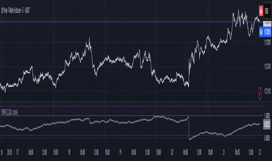
Aladin Pair Trading System v1Aladin Pair Trading System v1
What is This Indicator?
The Aladin Pair Trading System is a sophisticated tool designed to help traders identify profitable opportunities by comparing two related stocks that historically move together. Think of it as finding when one twin is running ahead or lagging behind the other - these moments often present trading opportunities as they tend to return to moving together.
Who Should Use This?
Beginners: Learn about statistical arbitrage and pair trading
Intermediate Traders: Execute mean-reversion strategies with confidence
Advanced Traders: Fine-tune parameters for optimal pair relationships
Portfolio Managers: Implement market-neutral strategies
💡 What is Pair Trading?
Imagine two ice cream shops next to each other. They usually have similar customer traffic because they're in the same area. If one day Shop A is packed while Shop B is empty, you might expect this imbalance to correct itself soon.
Pair trading works the same way:
You find two stocks that normally move together (like TCS and Infosys)
When one stock moves too far from the other, you trade expecting them to realign
You buy the lagging stock and sell the leading stock
When they come back together, you profit from both sides
Key Features
1. Z-Score Analysis
What it is: A statistical measure showing how far the price relationship has deviated from normal
What it means:
Z-Score near 0 = Normal relationship
Z-Score at +2 = Stock A is expensive relative to Stock B (Sell A, Buy B)
Z-Score at -2 = Stock A is cheap relative to Stock B (Buy A, Sell B)
2. Multiple Timeframe Analysis
Long-term Z-Score (300 bars): Shows the big picture trend
Short-term Z-Score (100 bars): Shows recent movements
Signal Z-Score (20 bars): Generates quick trading signals
3. Statistical Validation
The indicator checks if the pair is suitable for trading:
Correlation (must be > 0.7): Confirms the stocks move together
1.0 = Perfect positive correlation
0.7 = Strong correlation
Below 0.7 = Warning: pair may not be reliable
ADF P-Value (should be < 0.05): Tests if the relationship is stable
Low value = Good for pair trading
High value = Relationship may be random
Cointegration: Confirms long-term equilibrium relationship
YES = Pair tends to revert to mean
NO = Pair may drift apart permanently
Visual Elements Explained
Chart Zones (Color-Coded Areas)
Yellow Zone (-1.5 to +1.5)
Normal Zone: Relationship is stable
Action: Wait for better opportunities
Blue Zone (±1.5 to ±2.0)
Entry Zone: Deviation is significant
Action: Prepare for potential trades
Green/Red Zone (±2.0 to ±3.0)
Opportunity Zone: Strong deviation
Action: High-probability trade setups
Beyond ±3.0
Risk Limit: Extreme deviation
Action: Either maximum opportunity or structural break
Signal Arrows
Green Arrow Up (Buy A + Sell B):
Stock A is undervalued relative to B
Buy Stock A, Short Stock B
Red Arrow Down (Sell A + Buy B):
Stock A is overvalued relative to B
Sell Stock A, Buy Stock B
Settings Guide
Symbol Inputs
Pair Symbol (Symbol B): Choose the second stock to compare
Default: NSE:INFY (Infosys)
Example pairs: TCS/INFY, HDFCBANK/ICICIBANK, RELIANCE/ONGC
Z-Score Parameters
Long Z-Score Period (300): Historical context
Short Z-Score Period (100): Recent trend
Signal Period (20): Trading signals
Z-Score Threshold (2.0): Entry trigger level
Higher = Fewer but stronger signals
Lower = More frequent signals
Statistical Parameters
Correlation Period (240): How many bars to check correlation
Hurst Exponent Period (50): Measures mean-reversion tendency
Probability Lookback (100): Historical probability calculations
Trading Parameters
Entry Threshold (0.0): Minimum Z-score for entry
Risk Threshold (1.5): Warning level
Risk Limit (3.0): Maximum deviation to trade
How to Use (Step-by-Step)
Step 1: Choose Your Pair
Add the indicator to your chart (this becomes Stock A)
In settings, select Stock B (the comparison stock)
Choose stocks from the same sector for best results
Step 2: Verify Pair Quality
Check the Statistics Table (top-right corner):
✅ Correlation > 0.70 (Green = Good)
✅ ADF P-value < 0.05 (Green = Good)
✅ Cointegrated = YES (Green = Good)
If all three are green, the pair is suitable for trading!
Step 3: Wait for Signals
BUY SIGNAL (Green Arrow Up)
Z-Score crosses above -2.0
Action: Buy Stock A, Sell Stock B
Exit: When Z-Score returns to 0
SELL SIGNAL (Red Arrow Down)
Z-Score crosses below +2.0
Action: Sell Stock A, Buy Stock B
Exit: When Z-Score returns to 0
Step 4: Risk Management
Yellow Zone: Monitor only
Blue Zone: Prepare for entry
Green/Red Zone: Active trading zone
Beyond ±3.0: Maximum risk - use caution
⚠️ Important Warnings
Not All Pairs Work: Always check the statistics table first
Market Conditions Matter: Correlation can break during market stress
Use Stop Losses: Set stops at Z-Score ±3.5 or beyond
Position Sizing: Trade both legs with appropriate hedge ratios
Transaction Costs: Factor in brokerage and slippage for both stocks
Example Trade
Scenario: TCS vs INFOSYS
Correlation: 0.85 ✅
Z-Score: -2.3 (TCS is cheap vs INFY)
Action to be taken:
Buy 1lot of TCS Future
Sell 1lot of INFOSYS Future
Expected Outcome:
As Z-Score moves toward 0, TCS outperforms INFOSYS
Close both positions when Z-Score crosses 0
Profit from the convergence
Best Practices
Test Before Trading: Use paper trading first
Sector Focus: Choose pairs from the same industry
Monitor Statistics: Check correlation daily
Avoid News Events: Don't trade pairs during earnings/major news
Size Appropriately: Start small, scale with experience
Be Patient: Wait for high-quality setups (±2.0 or beyond)
What Makes This Indicator Unique?
Multi-timeframe Z-Score analysis: Three different perspectives
Statistical validation: Built-in correlation and cointegration tests
Visual risk zones: Easy-to-understand color-coded areas
Real-time statistics: Live pair quality monitoring
Beginner-friendly: Clear signals with educational zones
Technical Background
The indicator uses:
Engle-Granger Cointegration Test: Validates pair relationship
ADF (Augmented Dickey-Fuller) Test: Tests stationarity
Pearson Correlation: Measures linear relationship
Z-Score Normalization: Standardizes deviations
Log Returns: Handles price differences properly
Support & Community
For questions, suggestions, or to share your pair trading experiences:
Comment below the indicator
Share your successful pair combinations
Report any issues for quick fixes
Disclaimer
This indicator is for educational and informational purposes only. It does not constitute financial advice. Pair trading involves risk, including the risk of loss.
Always:
Do your own research
Understand the risks
Trade with money you can afford to lose
Consider consulting a financial advisor
📌 Quick Reference Card
Z-ScoreInterpretationAction-3.0 to -2.0A very cheap vs BStrong Buy A, Sell B-2.0 to -1.5A cheap vs BBuy A, Sell B-1.5 to +1.5Normal rangeHold/Wait+1.5 to +2.0A expensive vs BSell A, Buy B+2.0 to +3.0A very expensive vs BStrong Sell A, Buy B
Good Pair Statistics:
Correlation: > 0.70
ADF P-value: < 0.05
Cointegration: YES
Version: 1.0
Last Updated: 10th October 2025
Compatible: TradingView Pine Script v6
Happy Trading!

Technical Strength Index (TSI)📘 TSI with Dynamic Bands – Technical Strength Index
The TSI with Dynamic Bands is a multi-factor indicator designed to measure the statistical strength and structure of a trend. It combines several quantitative metrics into a single, normalized score between 0 and 1, allowing traders to assess the technical quality of market moves and detect overbought/oversold conditions with adaptive precision.
🧠 Core Components
This indicator draws from the StatMetrics library, blending:
📈 Trend Persistence: via the Hurst exponent, indicating whether price action is mean-reverting or trending.
📉 Risk-Adjusted Volatility: via the inverted , rewarding smoother, less erratic price movement.
🚀 Momentum Strength: using a combination of directional momentum and Z-score–normalized returns.
These components are normalized and averaged into the TSI line.
🎯 Features
TSI Line: Composite score of trend quality (0 = weak/noise, 1 = strong/structured).
Dynamic Bands: Mean ± 1 standard deviation envelopes provide adaptive context.
Overbought/Oversold Detection: Based on a rolling quantile (e.g. 90th/10th percentile of TSI history).
Signal Strength Bar (optional): Measures how statistically extreme the current TSI value is, helping validate confidence in trade setups.
Dynamic Color Cues: Background and bar gradients help visually identify statistically significant zones.
📈 How to Use
Look for overbought (red background) or oversold (green background) conditions as potential reversal zones.
Confirm trend strength with the optional signal strength bar — stronger values suggest higher signal confidence.
Use the TSI line and context bands to filter out noisy ranges and focus on structured price moves.
⚙️ Inputs
Lookback Period: Controls the smoothing and window size for statistical calculations.
Overbought/Oversold Quantiles: Adjust the thresholds for signal zones.
Plot Signal Strength: Enable or disable the signal confidence bar.
Overlay Signal Strength: Show signal strength in the same panel (compact) or not (cleaner TSI-only view).
🛠 Example Use Cases
Mean reversion traders identifying reversal zones with statistical backing
Momentum/Trend traders confirming structure before entries
Quantitative dashboards or multi-asset screening tools
⚠️ Disclaimer
This script is for educational and informational purposes only. It does not constitute financial advice or a recommendation to buy or sell any financial instrument.
This AI is not a financial advisor; please consult your financial advisor for personalized advice.
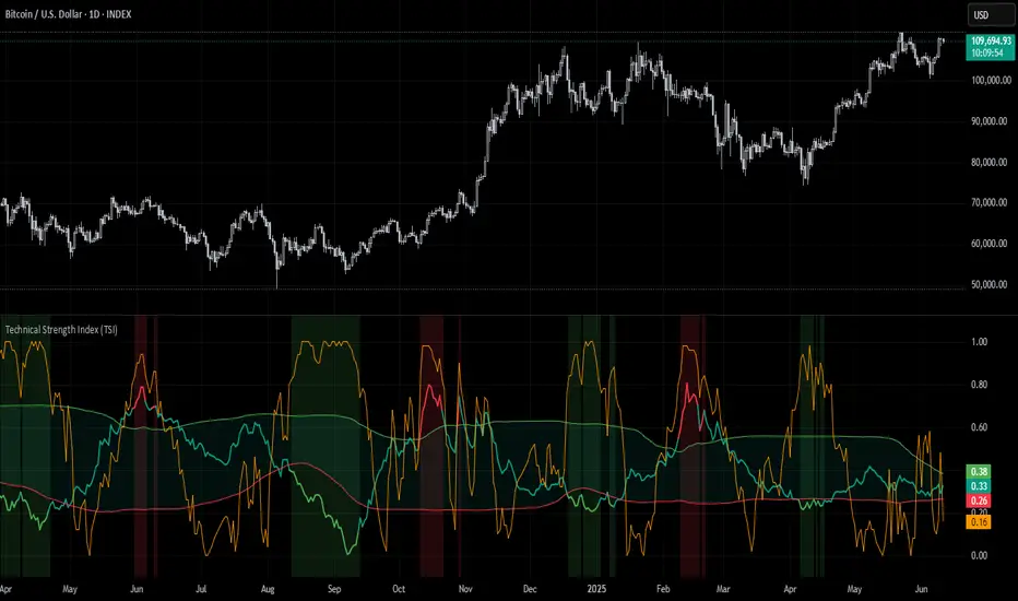
SCE ReversalsThis tool uses past market data to attempt to identify where changes in “memory” may occur to spot reversals. The Hurst Exponent was a big inspiration for this code. The main driver is identifying when past ranges expand and contract, leading to a change in direction. With the use of Sum of Squared Errors, users do not need to input anything.
Getting optimized parameters
// Define ranges for N and lkb
N_range = array.from(15, 20, 25, 30, 35, 40, 45, 50, 55, 60)
// Function to calculate SSE
sse_calc(_N) =>
x = math.pow(close - close , 2)
y = math.pow(close - close , 2) + math.pow(close, 2)
z = x / y
scaled_z = z * math.log(_N)
min_r = ta.lowest(scaled_z, _N)
max_r = ta.highest(scaled_z, _N)
norm_r = (scaled_z - min_r) / (max_r - min_r)
SMA = ta.sma(close, _N)
reversal_bullish = norm_r == 1.000 and norm_r < 0.90 and close < SMA and session.ismarket and barstate.isconfirmed
reversal_bearish = norm_r == 1.000 and norm_r < 0.90 and close > SMA and session.ismarket and barstate.isconfirmed
var float error = na
if reversal_bullish or reversal_bearish
error := math.pow(close - SMA, 2)
error
else
error := 999999999999999999999999999999999999999
error
error
var int N_opt = na
var float min_SSE = na
// Loop through ranges and calculate SSE
for N in N_range
sse = sse_calc(N)
if na(min_SSE) or sse < min_SSE
min_SSE := sse
N_opt := N
The N_range list encompasses every lookback value to check with. The sse_calc function accepts an individual element to then perform the calculation for Reversals. If there is a reversal, the error becomes how far away the close is from a moving average with that look back. Lowest error wins. That would be the look back used for the Reversals calculation.
Reversals calculation
// Calculating with optimized parameters
x_opt = math.pow(close - close , 2)
y_opt = math.pow(close - close , 2) + math.pow(close, 2)
z_opt = x_opt / y_opt
scaled_z_opt = z_opt * math.log(N_opt)
min_r_opt = ta.lowest(scaled_z_opt, N_opt)
max_r_opt = ta.highest(scaled_z_opt, N_opt)
norm_r_opt = (scaled_z_opt - min_r_opt) / (max_r_opt - min_r_opt)
SMA_opt = ta.sma(close, N_opt)
reversal_bullish_opt = norm_r_opt == 1.000 and norm_r_opt < 0.90 and close < SMA_opt and close > high and close > open and session.ismarket and barstate.isconfirmed
reversal_bearish_opt = norm_r_opt == 1.000 and norm_r_opt < 0.90 and close > SMA_opt and close < low and close < open and session.ismarket and barstate.isconfirmed
X_opt and y_opt are the compared values to develop the system. Everything done afterwards is scaling and using it to spot the Reversals. X_opt is the current close, minus the close with the optimal N bars back, squared. Then y_opt is also that but plus the current close squared. Z_opt is then x_opt / y_opt. This gives us a pretty small number that will go up when we approach tops or bottoms. To make life a little easier I normalize the value between 0 and 1.
After I find the moving average with the optimal N, I can check if there is a Reversal. Reversals are there when the last value is at 1 and the current value drops below 0.90. This would tell us that “memory” was strong and is now changing. To determine direction and help with accuracy, if the close is above the moving average it is a bearish alert, and vice versa. As well as the close must be below the last low for a bearish Reversal, above the last high for a bullish Reversal. Also the close must be above the open for a bullish Reversal, and below for a bearish one.
Visual examples
This NASDAQ:TSLA chart shows how alerts may come around. The bullish and bearish labels are plotted on the chart along with a reference line to see price interact with.
The indicator has the potential to be inactive, like we see here on $OKLO. There is only one alert, and it marks the bottom nicely.
Stocks with strong trends like NYSE:NOW may be more susceptible to false alerts. Assets that are volatile and bounce around a lot may be better.
It works on intra day charts the same as on Daily or longer charts. We see here on NASDAQ:QQQ it spotted the bottom on this particular trading day.
This tool is meant to aid traders in making decisions, not to be followed blindly. No trading tool is 100% accurate and Sum of Squared Errors does not guarantee the most optimal value. I encourage feedback and constructive criticism.

Moment-Based Adaptive DetectionMBAD (Moment-Based Adaptive Detection) : a method applicable to a wide range of purposes, like outlier or novelty detection, that requires building a sensible interval/set of thresholds. Unlike other methods that are static and rely on optimizations that inevitably lead to underfitting/overfitting, it dynamically adapts to your data distribution without any optimizations, MLE, or stuff, and provides a set of data-driven adaptive thresholds, based on closed-form solution with O(n) algo complexity.
1.5 years ago, when I was still living in Versailles at my friend's house not knowing what was gonna happen in my life tomorrow, I made a damn right decision not to give up on one idea and to actually R&D it and see what’s up. It allowed me to create this one.
The Method Explained
I’ve been wandering about z-values, why exactly 6 sigmas, why 95%? Who decided that? Why would you supersede your opinion on data? Based on what? Your ego?
Then I consciously noticed a couple of things:
1) In control theory & anomaly detection, the popular threshold is 3 sigmas (yet nobody can firmly say why xD). If your data is Laplace, 3 sigmas is not enough; you’re gonna catch too many values, so it needs a higher sigma.
2) Yet strangely, the normal distribution has kurtosis of 3, and 6 for Laplace.
3) Kurtosis is a standardized moment, a moment scaled by stdev, so it means "X amount of something measured in stdevs."
4) You generate synthetic data, you check on real data (market data in my case, I am a quant after all), and you see on both that:
lower extension = mean - standard deviation * kurtosis ≈ data minimum
upper extension = mean + standard deviation * kurtosis ≈ data maximum
Why not simply use max/min?
- Lower info gain: We're not using all info available in all data points to estimate max/min; we just pick the current higher and lower values. Lol, it’s the same as dropping exponential smoothing with alpha = 0 on stationary data & calling it a day.
You can’t update the estimates of min and max when new data arrives containing info about the matter. All you can do is just extend min and max horizontally, so you're not using new info arriving inside new data.
- Mixing order and non-order statistics is a bad idea; we're losing integrity and coherence. That's why I don't like the Hurst exponent btw (and yes, I came up with better metrics of my own).
- Max & min are not even true order statistics, unlike a percentile (finding which requires sorting, which requires multiple passes over your data). To find min or max, you just need to do one traversal over your data. Then with or without any weighting, 100th percentile will equal max. So unlike a weighted percentile, you can’t do weighted max. Then while you can always check max and min of a geometric shape, now try to calculate the 56th percentile of a pentagram hehe.
TL;DR max & min are rather topological characteristics of data, just as the difference between starting and ending points. Not much to do with statistics.
Now the second part of the ballet is to work with data asymmetry:
1) Skewness is also scaled by stdev -> so it must represent a shift from the data midrange measured in stdevs -> given asymmetric data, we can include this info in our models. Unlike kurtosis, skewness has a sign, so we add it to both thresholds:
lower extension = mean - standard deviation * kurtosis + standard deviation * skewness
upper extension = mean + standard deviation * kurtosis + standard deviation * skewness
2) Now our method will work with skewed data as well, omg, ain’t it cool?
3) Hold up, but what about 5th and 6th moments (hyperskewness & hyperkurtosis)? They should represent something meaningful as well.
4) Perhaps if extensions represent current estimated extremums, what goes beyond? Limits, beyond which we expect data not to be able to pass given the current underlying process generating the data?
When you extend this logic to higher-order moments, i.e., hyperskewness & hyperkurtosis (5th and 6th moments), they measure asymmetry and shape of distribution tails, not its core as previous moments -> makes no sense to mix 4th and 3rd moments (skewness and kurtosis) with 5th & 6th, so we get:
lower limit = mean - standard deviation * hyperkurtosis + standard deviation * hyperskewness
upper limit = mean + standard deviation * hyperkurtosis + standard deviation * hyperskewness
While extensions model your data’s natural extremums based on current info residing in the data without relying on order statistics, limits model your data's maximum possible and minimum possible values based on current info residing in your data. If a new data point trespasses limits, it means that a significant change in the data-generating process has happened, for sure, not probably—a confirmed structural break.
And finally we use time and volume weighting to include order & process intensity information in our model.
I can't stress it enough: despite the popularity of these non-weighted methods applied in mainstream open-access time series modeling, it doesn’t make ANY sense to use non-weighted calculations on time series data . Time = sequence, it matters. If you reverse your time series horizontally, your means, percentiles, whatever, will stay the same. Basically, your calculations will give the same results on different data. When you do it, you disregard the order of data that does have order naturally. Does it make any sense to you? It also concerns regressions applied on time series as well, because even despite the slope being opposite on your reversed data, the centroid (through which your regression line always comes through) will be the same. It also might concern Fourier (yes, you can do weighted Fourier) and even MA and AR models—might, because I ain’t researched it extensively yet.
I still can’t believe it’s nowhere online in open access. No chance I’m the first one who got it. It’s literally in front of everyone’s eyes for centuries—why no one tells about it?
How to use
That’s easy: can be applied to any, even non-stationary and/or heteroscedastic time series to automatically detect novelties, outliers, anomalies, structural breaks, etc. In terms of quant trading, you can try using extensions for mean reversion trades and limits for emergency exits, for example. The market-making application is kinda obvious as well.
The only parameter the model has is length, and it should NOT be optimized but picked consciously based on the process/system you’re applying it to and based on the task. However, this part is not about sharing info & an open-access instrument with the world. This is about using dem instruments to do actual business, and we can’t talk about it.
∞

Cycle OscillatorThe Cycle Oscillator is a tool developed to help traders analyze market cycles thanks to a simplified version of the Hurst theory and the easy visualization provided by the detrended cycle.
This indicator has two functions:
- The first one is the plotting of a line that oscillates above and below the zero line, which can be used to find the cycle direction and momentum
- The second feature is the next-cycle bottom forecaster, useful for estimating the timing of the future pivot low based on the pivot low of the oscillator.
This last feature shows graphically the period in which the next low will probably happen, using as a calculation method the timing of the previous indicator's lows.
Additionally, the user can choose to modify the cycle length to analyze bigger or smaller price movements.
This indicator can be greatly used in combination with other Cycle Indicators to gain more confluence in the plotted time areas.
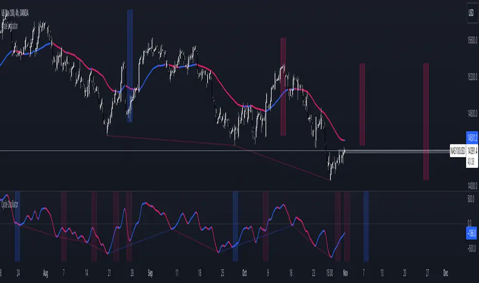
Cycle IndicatorThe Cycle Indicator is a tool developed to help traders analyze market cycles thanks to a simplified version of the Hurst theory.
This indicator has two functions:
- The first one is the plotting of a line that can be used to find the cycle direction and momentum
- The second feature is the next-cycle bottom forecaster, useful for estimating the timing of the future pivot low.
This last feature shows graphically the period in which the next low will probably happen, using as a calculation method the timing of the previous lows.
Additionally, the user can choose to extend this time zone or to limit them to the range between the last pivot high and low.

[blackcat] L2 Fourier Series AnalysisLevel 2
Background
John Ehlers’ articles in the July issues on 2019,“Fourier Series Model Of The Market”.
Function
In “Fourier Series Model Of The Market” in this issue, author John Ehlers introduces a Fourier series indicator designed to help traders identify cycles in the market. According to the author, the approach based on five principles outlined by J.M. Hurst in his 1970 book allows the determinization of a security’s primary cycle period and gives a faithful picture of market activity.
Remarks
You have to adjust Entry_TH value for different time frames.
Feedbacks are appreciated.

Rescaled RangeRescaled Range is an implementation of the fractal rescaled ranges developed by Harold Edwin Hurst and Benoit Mandlebrot.
Settings include:
“Window Size” - the number of time periods in a window over which price changes are analyzed. This will generally correspond to your trading horizon and defaults to 15.
“Number of Windows” - the number of “Window Size” intervals to average the rescaled range value over. By looking at a number of such periods, the study captures potential volatility that may have occurred in the recent past. This should be set long enough to capture the current trend (defaults to 63), but not so long to include volatility regimes no longer in play.
Each window in the average is offset by 1 time period from the the others - like a moving average.
This study plots two lines - “Rescaled Range High” which indicates overbought conditions when the price moves above it and “Rescaled Range Low” which indicates oversold conditions when the price moves below it.
This study builds upon the bridge range work of Joe Catanzaro (joecat808) and Caleb Sandfort (calebsandfort). Bridge ranges are used to position the rescaled range with respect to the closing price.
Note: Your time series must have (Window Size + Number of Windows) or more periods of data to complete this study. For example, using the defaults, your time series should have (15+63) = 78 periods or more of data.
