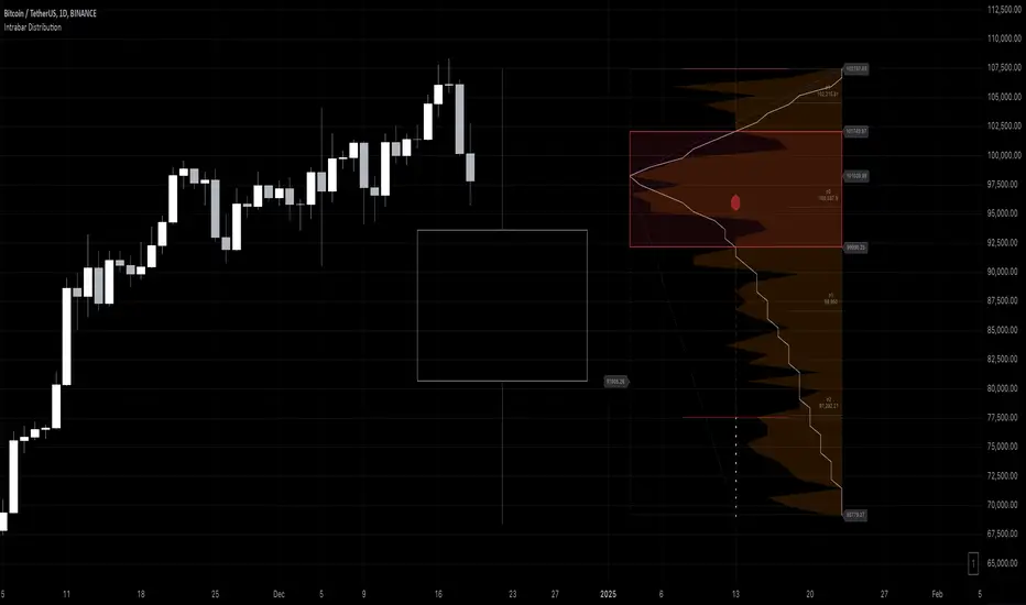
Intrabar DistributionThe Intrabar Distribution publication is an extension of the Intrabar BoxPlot publication. Besides a boxplot, it showcases price and volume distribution using intrabar Lower Timeframe (LTF) values (close) which can be displayed on the chart or in a separate pane.
🔶 USAGE
Intrabar Distribution has several features, users can display:
Recent candle for comparison against the other features
Boxplot of recent candle
Price distribution (optionally displayed as a curve)
Volume distribution
🔹 Recent candle / Boxplot
The middle 50% intrabar close values (Interquartile range, or IQR) are shown as a box, where the upper limit is percentile 75 (p75), and the lower limit is percentile 25 (p25). The dashed lines show the addition/subtraction of 1.5*IQR. All values out of range are considered outliers. They are displayed as white dots within the IQR*1.5 range or white X's when beyond the IQR*3 range (extreme outliers).
By showing the middle 50% intrabar values through a box, we can more easily see where the intrabar activity is mainly situated.
Note in the example above an upward-directed candle with a negative volume delta, displayed as a red box and dot (see further).
As seen in the following example, compared against the recent candle (grey candle at the left), most of the intrabar activity lies just beneath the opening price.
Note that results will be more accurate when more data is available, which can be done by making the difference between the current timeframe and the intrabar timeframe large enough.
🔹 Price / Volume distribution
The price and volume distribution can be helpful for highlighting areas of interest.
Here, we can see two areas where intrabar closing prices are mainly positioned.
The following example shows three successive bars. The recent bar is displayed on the left side, together with the volume distribution. The boxplot and price distribution are displayed on the right.
You can see the difference between volume and price distribution.
At the first bar, most price activity is at the top, while most of the volume was generated at the bottom; in other words, the price got briefly in the bottom region, with high volume before it returned.
At the second bar, price and volume are relatively equally distributed, which fits for indecisiveness.
The third bar shows more volume at a higher region; most intrabar closing prices are above the closing price.
Following example shows the same with 'Curve shaped' enabled (Settings: 'Price Distribution')
When 'Curve shaped' is enabled, lines/labels are shown with the standard deviation distance.
A blue 'guide line' can be enabled for easier interpretation.
🔹 Volume Delta
When there is a discrepancy between the delta volume and direction of the candle, this will be displayed as follows:
Red candle: when the sum of the volume of green intrabars is higher than the sum of the volume of red intrabars, the 'mean dot' will be coloured green.
Green candle: when the sum of the volume of red intrabars is higher than the sum of the volume of green intrabars, the 'mean dot' will be coloured red.
🔶 DETAILS
The intrabar values are sorted and split in parts/sections. The number of values in each section is displayed as a white line
The same principle applies to volume distribution, where the sum of volume per section is displayed as an orange area.
The boxplot displays several price values
Last close price
Highest / lowest intrabar close price
Median
p25 / p75
🔹 LTF settings
When 'Auto' is enabled (Settings, LTF), the LTF will be the nearest possible x times smaller TF than the current TF. When 'Premium' is disabled, the minimum TF will always be 1 minute to ensure TradingView plans lower than Premium don't get an error.
Examples with current Daily TF (when Premium is enabled):
500 : 3 minute LTF
1500 (default): 1 minute LTF
5000: 30 seconds LTF (1 minute if Premium is disabled)
🔶 SETTINGS
Location: Chart / Pane (when pane is opted, move the indicator to a separate pane as well)
Parts: divides the intrabar close values into parts/sections
Offset: offsets every drawing at once
Width: width of drawings, only applicable on "location: chart"
Label size: size of price labels
🔹 LTF
LTF: LTF setting
Auto + multiple: Adjusts the initial set LTF
Premium: Enable when your TradingView plan is Premium or higher
🔹 Current Bar
Display toggle + color setting
Offset: offsets only the 'Current Bar' drawing
🔹 Intrabar Boxplot
Display toggle + Colors, dependable on different circumstances.
Up: Price goes up, with more bullish than bearish intrabar volume.
Up-: Price goes up, with more bearish than bullish intrabar volume.
Down: Price goes down, with more bearish than bullish intrabar volume.
Down+: Price goes down, with more bullish than bearish intrabar volume.
Offset: offsets only the 'Boxplot' drawing
🔹 Price distribution
Display toggle + Color.
Curve Shaped
Guide Lines: Display 2 blue lines
Display Price: Show price of 'x' standard deviation
Offset: offsets only the 'Price distribution' drawing
Label size: size of price labels (standard deviation)
🔹 Volume distribution
Display toggle + Color.
Offset: offsets only the 'Volume distribution' drawing
🔹 Table
Show TF: Show intrabar Timeframe.
Textcolor
Size Table: Text Size
Wyszukaj w skryptach "curve"
EMD Oscillator (Zeiierman)█ Overview
The Empirical Mode Decomposition (EMD) Oscillator is an advanced indicator designed to analyze market trends and cycles with high precision. It breaks down complex price data into simpler parts called Intrinsic Mode Functions (IMFs), allowing traders to see underlying patterns and trends that aren’t visible with traditional indicators. The result is a dynamic oscillator that provides insights into overbought and oversold conditions, as well as trend direction and strength. This indicator is suitable for all types of traders, from beginners to advanced, looking to gain deeper insights into market behavior.
█ How It Works
The core of this indicator is the Empirical Mode Decomposition (EMD) process, a method typically used in signal processing and advanced scientific fields. It works by breaking down price data into various “layers,” each representing different frequencies in the market’s movement. Imagine peeling layers off an onion: each layer (or IMF) reveals a different aspect of the price action.
⚪ Data Decomposition (Sifting): The indicator “sifts” through historical price data to detect natural oscillations within it. Each oscillation (or IMF) highlights a unique rhythm in price behavior, from rapid fluctuations to broader, slower trends.
⚪ Adaptive Signal Reconstruction: The EMD Oscillator allows traders to select specific IMFs for a custom signal reconstruction. This reconstructed signal provides a composite view of market behavior, showing both short-term cycles and long-term trends based on which IMFs are included.
⚪ Normalization: To make the oscillator easy to interpret, the reconstructed signal is scaled between -1 and 1. This normalization lets traders quickly spot overbought and oversold conditions, as well as trend direction, without worrying about the raw magnitude of price changes.
The indicator adapts to changing market conditions, making it effective for identifying real-time market cycles and potential turning points.
█ Key Calculations: The Math Behind the EMD Oscillator
The EMD Oscillator’s advanced nature lies in its high-level mathematical operations:
⚪ Intrinsic Mode Functions (IMFs)
IMFs are extracted from the data and act as the building blocks of this indicator. Each IMF is a unique oscillation within the price data, similar to how a band might be divided into treble, mid, and bass frequencies. In the EMD Oscillator:
Higher-Frequency IMFs: Represent short-term market “noise” and quick fluctuations.
Lower-Frequency IMFs: Capture broader market trends, showing more stable and long-term patterns.
⚪ Sifting Process: The Heart of EMD
The sifting process isolates each IMF by repeatedly separating and refining the data. Think of this as filtering water through finer and finer mesh sieves until only the clearest parts remain. Mathematically, it involves:
Extrema Detection: Finding all peaks and troughs (local maxima and minima) in the data.
Envelope Calculation: Smoothing these peaks and troughs into upper and lower envelopes using cubic spline interpolation (a method for creating smooth curves between data points).
Mean Removal: Calculating the average between these envelopes and subtracting it from the data to isolate one IMF. This process repeats until the IMF criteria are met, resulting in a clean oscillation without trend influences.
⚪ Spline Interpolation
The cubic spline interpolation is an advanced mathematical technique that allows smooth curves between points, which is essential for creating the upper and lower envelopes around each IMF. This interpolation solves a tridiagonal matrix (a specialized mathematical problem) to ensure that the envelopes align smoothly with the data’s natural oscillations.
To give a relatable example: imagine drawing a smooth line that passes through each peak and trough of a mountain range on a map. Spline interpolation ensures that line is as smooth and close to reality as possible. Achieving this in Pine Script is technically demanding and demonstrates a high level of mathematical coding.
⚪ Amplitude Normalization
To make the oscillator more readable, the final signal is scaled by its maximum amplitude. This amplitude normalization brings the oscillator into a range of -1 to 1, creating consistent signals regardless of price level or volatility.
█ Comparison with Other Signal Processing Methods
Unlike standard technical indicators that often rely on fixed parameters or pre-defined mathematical functions, the EMD adapts to the data itself, capturing natural cycles and irregularities in real-time. For example, if the market becomes more volatile, EMD adjusts automatically to reflect this without requiring parameter changes from the trader. In this way, it behaves more like a “smart” indicator, intuitively adapting to the market, unlike most traditional methods. EMD’s adaptive approach is akin to AI’s ability to learn from data, making it both resilient and robust in non-linear markets. This makes it a great alternative to methods that struggle in volatile environments, such as fixed-parameter oscillators or moving averages.
█ How to Use
Identify Market Cycles and Trends: Use the EMD Oscillator to spot market cycles that represent phases of buying or selling pressure. The smoothed version of the oscillator can help highlight broader trends, while the main oscillator reveals immediate cycles.
Spot Overbought and Oversold Levels: When the oscillator approaches +1 or -1, it may indicate that the market is overbought or oversold, signaling potential entry or exit points.
Confirm Divergences: If the price movement diverges from the oscillator's direction, it may indicate a potential reversal. For example, if prices make higher highs while the oscillator makes lower highs, it could be a sign of weakening trend strength.
█ Settings
Window Length (N): Defines the number of historical bars used for EMD analysis. A larger window captures more data but may slow down performance.
Number of IMFs (M): Sets how many IMFs to extract. Higher values allow for a more detailed decomposition, isolating smaller cycles within the data.
Amplitude Window (L): Controls the length of the window used for amplitude calculation, affecting the smoothness of the normalized oscillator.
Extraction Range (IMF Start and End): Allows you to select which IMFs to include in the reconstructed signal. Starting with lower IMFs captures faster cycles, while ending with higher IMFs includes slower, trend-based components.
Sifting Stopping Criterion (S-number): Sets how precisely each IMF should be refined. Higher values yield more accurate IMFs but take longer to compute.
Max Sifting Iterations (num_siftings): Limits the number of sifting iterations for each IMF extraction, balancing between performance and accuracy.
Source: The price data used for the analysis, such as close or open prices. This determines which price movements are decomposed by the indicator.
-----------------
Disclaimer
The information contained in my Scripts/Indicators/Ideas/Algos/Systems does not constitute financial advice or a solicitation to buy or sell any securities of any type. I will not accept liability for any loss or damage, including without limitation any loss of profit, which may arise directly or indirectly from the use of or reliance on such information.
All investments involve risk, and the past performance of a security, industry, sector, market, financial product, trading strategy, backtest, or individual's trading does not guarantee future results or returns. Investors are fully responsible for any investment decisions they make. Such decisions should be based solely on an evaluation of their financial circumstances, investment objectives, risk tolerance, and liquidity needs.
My Scripts/Indicators/Ideas/Algos/Systems are only for educational purposes!

VIX Futures Spread StrategyThis script was an exercise in learning Pinescript and exploring the futures curve of the VIX in relation to SPY. Was deleted by TV, trying to republish it now with updated parameters for slippage and commission and a more detailed description.
"VIX Futures Spread Strategy" is a trading strategy that capitalizes on the spread between the 3-month VIX futures (VIX3M) and the spot VIX index. This strategy is based on the idea that the VIX futures spread can serve as a contrarian indicator of market sentiment, with extreme negative spreads potentially signaling oversold conditions and opportunities for long positions.
Ordinarily the VIX curve is in contango as futures contracts are priced at a premium to the current spot price and are used to hedge future uncertainty in the market. When the spot price of VIX spikes the curve can invert and enter backwardation; this strategy detects this condition and uses it as a trigger to open a long position in SPY. The spread going negative tends to correlate with excessive fear and uncertainty in the short term while expecting lower volatility in the long term, in this case 3 months out.
The strategy is designed to enter a long position when the VIX futures spread is negative and to exit the position when the spread rises above 3 -- when the curve is in contango again. The strategy employs a pyramiding approach, allowing up to 10 additional orders to be placed while the entry condition is met, with each order consisting of 10 contracts. This approach aims to maximize potential profits during periods of favorable market conditions.
In this strategy, the VIX futures spread is calculated as the difference between the 3-month VIX futures (VIX3M) and the spot VIX index. The spread is plotted as a histogram on the chart, with the zero line representing no spread, and horizontal lines at 0 and 3 indicating the entry and exit thresholds, respectively.
The strategy's backtesting settings use an initial capital of HKEX:10 ,000, a commission of 0.5% per trade, and a maximum of 10 pyramiding orders, and a slippage of 2 ticks.
Please note that this strategy is intended for educational purposes and should not be considered as financial advice. Before using this strategy in live trading, make sure to thoroughly test and optimize its parameters to suit your risk tolerance and specific trading conditions.

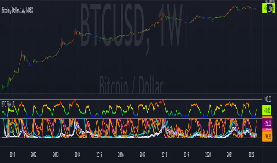
Bitcoin Risk Long Term indicatorOBJECTIVE:
The purpose of this indicator is to synthesize via an average several indicators from a wide choice with in order to simplify the reading of the bitcoin price and that on a long term vision.
Useful for those who want to see things simply, typically to make a smart DCA based on risk.
I originally used this script as a sandbox to understand and test the usefulness of several indicators, and to develop my PineScript skills, but finally the Risk Indicator output seems relevant so I decided to share it.
USAGE:
The selected indicators are the ones that I think give the best market bottoms, but the idea here is that anyone can try and use any set of indicators based on those preferences (post in comments if you find a relevant config)
Most of the indicator inputs are configurable. And some are not taken into account in the calculation of the Risk indicator because I consider them not relevant, this script is also a test more than a final version.
NOTES :
If you have any idea of adding an indicator, modification, criticism, bug found: share them, it is appreciated!
In the future I will create another more versatile Risk indicator that will not be focused on bitcoin in weekly. (this indicator is still usable on other assets and timeframe)
THANKS:
to Benjamin Cowen for inspiring me with his Bitcoin Risk metric
to Lazybear for his Wavetrend Indicator and all the scripts he shares
to Mabonyi for his Bitcoin Logarithmic Growth Curves & Zones script
to VuManChu for his VMC Cypher B Divergence
to the Trading view team for developing TV and PineScript
And to all the community for all the published codes that allowed me to progress and create this script
---- FR ----
OBJECTIF :
L'objectif de cet indicateur est de synthétiser via une moyenne plusieurs indicateurs parmi un large choix avec afin de simplifier la lecture du cours de bitcoin et cela sur une vision longue terme.
Utile pour ceux qui veulent voir les choses simplement, typiquement faire un DCA intelligent en fonction du risque.
À la base j'ai utilisé ce script comme un bac à sable pour comprendre puis tester l'utilité de plusieurs indicateurs, et développer mes compétences PineScript, mais finalement l'output Risk Indicateur me semble pertinent donc autant le partager.
UTILISATION :
Les indicateurs sélectionnés sont ceux qui permettent selon moi d'avoir les meilleurs point bas de marché, mais l'idée ici est que chacun puisse essayer et utiliser n'importe quel ensemble d'indicateur en fonction de ces préférences (poster en commentaire si vous trouvez une configuration pertinente)
La plupart des inputs indicateurs sont paramétrables. Et certains ne sont pas pris en compte dans le calcul du Risk indicateur car je les estime non pertinent, ce script est aussi un essai plus qu'une version finale.
NOTES :
Si vous avez la moindre idée d'ajout d'indicateur, modification, critique, bug trouvé : partagez-les, c'est apprécié !
à l'avenir je créerais un autre Risk indicator plus polyvalent qui ne sera pas focalisé sur bitcoin en weekly. (cet indicateur est tout de même utilisable sur d'autre actif et timeframe)
REMERCIEMENT :
à Benjamin Cowen pour m'avoir inspiré avec son Bitcoin Risk metric
à Lazybear pour son Wavetrend Indicator et globalement tout les scripts qu'il partage
à Mabonyi pour son script Bitcoin Logarithmic Growth Curves & Zones
à VuManChu pour son VMC Cypher B Divergence
à l'équipe Trading view pour avoir développé TV et PineScript
Et à toute la communauté pour tous les codes publiés qui m'ont permis de progresser et de créer ce script
[blackcat] L2 Hann Ehanced DMILevel: 2
Background
Among the many indicators, it can be said that DMI is the only "super turning" indicator. This indicator can alone send out risk warning signals when extreme market conditions occur in the stock market, helping us to solve some problems.
If we can operate according to the instructions of DMI, firstly, we can avoid the mistake of buying stocks at the head. Secondly, in the process of falling fear of the market, we can follow the direction signal sent by DMI and catch every time on the way down. Opportunity to rebound to unwind.
If you look at the diagram of the DMI, you will think it is very complicated, because there are four lines in its diagram, and they are intertwined, and it is difficult to distinguish the complex signals in it. But don't worry about its complex structure, we will fully dissect this indicator.
Function
These four lines are: PDI, MDI, ADX and ADXR. The scale of the table is from 0-100, which means from very weak to very strong. The PDI curve and MDI curve on some software are called +DI curve and -DI curve , all have the same meaning.
PDI: Represents the position of multiple parties in the market.
In market movements, the higher the PDI, the stronger the current market. On the contrary, it is a weak market. The A-share market is easy to go to extremes. Therefore, we can see that in the past A-share market, the PDI sometimes fell to near zero, and at this time, it often indicated that a rebound and uptrend was about to start.
MDI: Represents the position of the bears in the market.
In the market movement, the higher the MDI goes, the weaker the current market is, and vice versa, it is a strong market. Before a big bull market comes, we can see the MDI drop to a position close to zero, and at this time, the bears in the market have no power to fight back.
The relationship between PDI and MDI:
In the operation of the market, PDI and MDI are intertwined with each other. If the PDI is above the MDI, the market at this time is a strong market. The MDI is above the PDI, which is a bear market. The closer the distance between the two, the market is in a stalemate of consolidation. On the contrary, the further apart the two lines are, the more obvious the unilateral nature of the market is, whether it is a bull market or a bear market. The so-called unilateral market means that there is no midway adjustment when it rises, and there is no rebound correction when it falls.
ADX: Fast steering pullback.
The difference between ADX and other analysis indicators is that whether it is rising or falling, as long as there is a unilateral market, it runs upwards, not like other indicators, the strong market runs upwards and the weak market runs downwards.
The thread is almost entwined with PDI and MDI in general market movement, which makes no sense at this time. However, once the market breaks out of the market and starts to go to extremes, whether the market is rising or falling, ADX will start to run upwards. At this time, ADX has a clear meaning, because DMI has begun to issue early warning of impending turn!
ADXR: slow pull back.
This line is matched to ADX and is a moving average of ADX values. When ADX goes up, ADXR goes up with it, just slower.
When a round of rapid decline ends, it usually needs to be corrected by a rebound, and ADX will take the lead in turning up. Once it crosses with ADXR, it is regarded as an effective breakthrough.
Numerical division. I set an input threshold for HEDMI, and users can set the optimal threshold to buy and sell according to different TFs.
When PDI crosses the threshold, no matter how strong the bull market is, we must beware of risks from happening at any time.
In order to distinguish more clearly, I slightly modified the formula of the system, and when this happens, the indicator will issue a green warning label, so as to avoid risks in time.
Comprehensive use of four lines:
If the four lines in the steering indicator DMI are intertwined below 50, it usually means that the market is in a state of mild consolidation at this time. The DMI indicator at this time is useless because it does not generate a strong pullback force. Don't worry about an unexpected turnaround in the market. As for the consolidation, it's not a turnaround, it's a breakout.
When PDI and MDI gradually separate, at this time, ADX and ADXR will also rise. At this time, the DIM that is usually messy like twine will be clearly separated. When rising, PDI rises along with ADX and ADXR, while MDI sinks weakly. On the contrary, when the market starts to fall, MDI will rise along with ADX and ADXR, and PDI will sink helplessly. At this time, the DMI will be like a "tiger's mouth", gradually opening its bloody mouth. The bigger the opening, the more lethal the bite.
Here comes a tactic, or technical trend, called double hooves, that is, PDI and MDI split, ADX and ADXR upward to produce golden forks, PDI and MDI are like the double front hooves of a horse, ADX and ADXR The golden fork is like the rear hooves of a steed ready to take off, and this trend of the four lines is like the four legs of a steed that is about to run.
If you think it is too complicated to look at DMI like this, then I can tell you the easiest way to judge, that is, just look at the PDI line. When the PDI line falls below 10, boldly buy the dip, because it is a dip, so you need to calculate the rebound At this time, combined with the golden section theory I often talk about, you can easily find the selling point by making the golden section of the downward trend for the previous trend.
This kind of bottom-hunting method uses the golden section theory, and basically there will be no losses. Remember that one thing is not to be greedy and strictly enforce discipline. This is bottom-hunting, and advancing with both hooves is chasing up. The two styles are different, and the operation styles are different. You also need to explore more in actual combat. Any kind of trick, if you practice it proficiently, it is a unique trick.
Remark
Hanning Window Enhanced DMI
Free and Open Source Indicator

72s Strat: Backtesting Adaptive HMA+ pt.1This is a follow up to my previous publication of Adaptive HMA+ few months ago, as a mean to provide some kind of initial backtesting tools. Which can be use to explore many possible strategies, optimise its settings to better conform user's pair/tf, and hopefully able to help tweaking your general strategy.
If you haven't read the study or use the indicator, kindly go here first to get the overall idea.
The first strategy introduce in this backtest is one most basic already described in the study; buy/sell is when movement is there and everything is on the right side; When RSI has turned to other side, we can use it as exit point (if in profit of course, else just let it hit our TP/SL, why would we exit before profit). Also, base on RSI when we make entry, we can further differentiate type of signals. --Please check all comments in code directly where the signals , entries , and exits section are.
Second additional strategy to check; is when we also use second faster Adaptive HMA+ for exit. So this is like a double orders on a signal but with different exit-rule (/more on this on snapshots below). Alternatively, you can also work the code so to only use this type of exit.
There's also an additional feature which you can enable its visuals, the Distance Zone , is to help measuring price distance to our xHMA+. It's just a simple atr based envelope really, I already put the sample code in study's comment section, but better gonna update it there directly for non-coder too, after this.
In this sample I use Lot for order quantity size just because that's what I use on my broker. Also what few friends use while we forward-testing it since the study is published, so we also checked/compared each profit/loss report by real number. To use default or other unit of measurement, change the entry code accordingly.
If you change your order size, you should also change the commission in Properties Tab. My broker commission is 5 USD per order/lot, so in there with example order size 0.1 lot I put commission 0.5$ per order (I'll put 2.5$ for 0.5 lot, 10$ for 2 lot, and so on). Crypto usually has higher charge. --It is important that you should fill it base on your broker.
SETTINGS
I'm trying to keep it short. Please explore it further again. (Beginner should also first get acquaintance with terms use here.)
ORDERS:
Base Minimum Profit Before Exit:
The number is multiplier of ongoing ATR. Means that when basic exit condition is met, algo will check whether you're already in minimum profit or not, if not, let it still run to TP or SL, or until it meets subsequent exit condition, then it will check again.
Default Target Profit:
Multiplier of ATR at signal. If reached before any eligible exit condition is met, exit TP.
Base StopLoss Point:
You can change directly in code to use other like ATR Trailing SL, fix percent SL, or whatever. In the sample, 4 options provided.
Maximum StopLoss:
This is like a safety-net, that if at some point your chosen SL point from input above happens to be exceeding this maximum input that you can tolerate, then this max point is the one will be use as SL.
Activate 2nd order...:
The additional doubling of certain buy/sell with different exits as described above. If enable, you should also set pyramiding to at least: 2. If not, it does nothing.
ADAPTIVE HMA+ PERIOD
Many users already have their own settings for these. So in here I only sample the default as first presented in the study. Make it to your adaptive.
MARKET MOVEMENT
(1) Now you can check in realtime how much slope degree is best to define your specific pair/tf is out of congestion (yellow) area. And (2) also able to check directly what ATR lengths are more suitable defining your pair's volatility.
DISTANCE ZONE
Distance Multiplier. Each pair/tf has its own best distance zone (in xHMA+ perspective). The zone also determine whether a signal should appear or not. (Or what type of signal, if you wanna go more detail in constructing your strategy)
USAGE
(Provided you already have your own comfortable settings for minimum-maximum period of Adaptive HMA+. Best if you already have backtested it manually too and/or apply as an add-on to your working strategy)
1. In our experiences, first most important to define is both elements in the Market Movement Settings . These also tend to be persistent for whole season since it's kinda describing that pair/tf overall behaviour. Don't worry if you still get a low Profit Factor here, but by tweaking you should start to see positive changes in one of Max Drawdown and Net Profit, or Percent Profitable.
2. Afterwards, find your pair/tf Distance Zone . When optimising this, what we seek is just a "not to bad" equity curves to start forming. At least Max Drawdown should lessen more. Doesn't have to be great already, but should be better, no red in Net Profit.
3. Then go manage the "Trailing Minimum Profit", TP, SL, and max SL.
4. Repeat 1,2,3. 👻
5. Manage order size, commission, and/or enable double-order (need pyramiding) if you like. Check if your equity can handle max drawdown before margin call.
6. After getting an acceptable backtest result, go to List of Trades tab and find the biggest loss or when many sequencing loss in a row happened. Click on it to go to exact point on chart, observe why the signal failed and get at least general idea how it can be prevented . The rest is yours, you should know your pair/tf more than other.
You can also re-explore your minimum-maximum period for both Major and minor xHMA+.
Keep in mind that all numbers in Setting are conceptually in a form of range . You don't want to get superb equity curves but actually a "fragile" , means one can easily turn it to disaster just by changing only a fraction in one/two of the setting.
---
If you just wanna test the strength of the indicator alone, you can disable "Use StopLoss" temporarily while optimising settings.
Using no SL might be tempting in overall result data in some cases, but NOTE: It is not recommended to not using SL, don't forget that we deliberately enter when it's in high volatility. If want to add flexibility or trading for long-term, just maximise your SL. ie.: chose SL Point>ATR only and set it maximum. (Check your max drawdown after this).
I think this is quite important specially for beginners, so here's an example; Hypothetically in below scenario, because of some settings, the buy order after the loss sell signal didn't appear. Let's say if our initial capital only 1000$ using leverage and order size 0,5 lot (risky position sizing already), moreover if this happens at the beginning of your trading season, that's half of account gone already in one trade . Your max SL should've made you exit after that pumping bar.
The Trailing Minimum Profit is actually look like this. Search in the code if you want to plot it. I just don't like too many lines on chart.
To maximise profit we can try enabling double-order. The only added rule coded is: RSI should rising when buy and falling when sell. 2nd signal will appears above or below default buy/sell signal. (Of course it's also prone to double-loss, re-check your max drawdown after. Profit factor play its part in here for a long run). Snapshot in comparison:
Two default sell signals on left closed at RSI exit, the additional sell signal closed later on when price crossover minor xHMA+. On buy side, price haven't met our minimum profit when first crossunder minor xHMA+. If later on we hit SL on this "+buy" signal, at least we already profited from default buy signal. You can also consider/treat this as multiple TP points.
For longer-term trading, what you need to maximise is the Minimum Profit , so it won't exit whenever an exit condition happened, it can happen several times before reaching minimum profit. Hopefully this snapshot can explain:
Notice in comparison default sell and buy signal now close in average after 3 days. What's best is when we also have confirmation from higher TF. It's like targeting higher TF by entering from smaller TF.
As also mention in the study, we can still experiment via original HMA by putting same value for minimum-maximum period setting. This is experimental EU 1H with Major xHMA+: 144-144, Flat market 13, Distance multiplier 3.6, with 2nd order activated.
Kiwi was a bit surprising for me. It's flat market is effectively below 6, with quite far distance zone of 3.5. Probably because I'm using big numbers in adaptive period.
---
The result you see in strategy tester report below for EURUSD 15m is using just default settings you see in code, as follow:
0,1 lot for each order (which is the smallest allowed by my broker).
No pyramiding. Commission: 0.5 usd per order. Slippage: 3
Opening position is only using basic strategy #1 (RSI exit). Additional exit not activated.
Minimum Profit: 1. TP: 3.
SL use: Half-distance zone. Max SL: 4.5.
Major xHMA+: 172-233. minor xHMA+: 89-121
Distance Zone Multiplier: 2.7
RSI: Standard 14.
(From our forward-testing, the difference we get from net profit is because of the spread, our entry isn't exactly at the close/open price. Not so much though, but not the same. If somebody can direct me to any example where we can code our entry via current bid/ask price, that would be awesome!)
It's already a long post (sorry), think I'm gonna pause here. Check out the code :)
---
DISCLAIMER: Past performance is no guarantee of future results , and so on.. you know the drill ;)
Please read whole description first before using, don't take 1-2 paragraph and claim it's the whole logic, you are responsible of your own actions and understanding.

Recession IndicatorThis script attempts to predict recessions four quarters ahead.
According to the New York Fed, "The yield curve—specifically, the spread between the interest rates on the ten-year Treasury
note and the three-month Treasury bill—is a valuable forecasting tool. It is simple to use
and significantly outperforms other financial and macroeconomic indicators in predicting
recessions two to six quarters ahead."
The paper offers Estimated Recession Probabilities Using the Yield Curve Spread:
Four Quarters Ahead
Recession Probability Value of Spread
(Percent) (Percentage Points)
5 1.21
10 0.76
15 0.46
20 0.22
25 0.02
30 -0.17
40 -0.50
50 -0.82
60 -1.13
70 -1.46
80 -1.85
90 -2.40
"Note: The yield curve spread is defined as the spread between the
interest rates on the ten-year Treasury note and the three-month
Treasury bill."
You can choose at which Recession Probability (percent) you want to display the signal (default value is 25%), as well as choose if you want to only display the signal at inversion (default) or at all times when the yield curve is inverted.
To use, just select your current timeframe from the menu.
Includes an option for repainting -- default value is true, meaning the script will repaint the current bar.
False = Not Repainting = Value for the current bar is not repainted, but all past values are offset by 1 bar.
True = Repainting = Value for the current bar is repainted, but all past values are correct and not offset by 1 bar.
In both cases, all of the historical values are correct, it is just a matter of whether you prefer the current bar to be realistically painted and the historical bars offset by 1, or the current bar to be repainted and the historical data to match their respective price bars.
As explained by TradingView,`f_security()` is for coders who want to offer their users a repainting/no-repainting version of the HTF data.

Right Sided Ricker Moving Average And The Gaussian DerivativesIn general gaussian related indicators are built by using the gaussian function in one way or another, for example a gaussian filter is built by using a truncated gaussian function as filter kernel (kernel refer to the set weights) and has many great properties, note that i say truncated because the gaussian function is not supposed to be finite. In general the gaussian function is represented by a symmetrical bell shaped curve, however the gaussian function is parametric, and the user might adjust the position of the peak as well as the width of the curve, an indicator using this parametric approach is the Arnaud Legoux moving average (ALMA) who posses a length parameter controlling the filter length, a peak parameter controlling the position of the peak of the gaussian function as well as a width parameter, those parameters can increase/decrease the lag and smoothness of the moving average output.
However what about the derivatives of the gaussian function ? We don't talk much about them and thats a pity because they are extremely interesting and have many great properties as well, therefore in this post i'll present a low lag moving average based on the modification of the 2nd order derivative of the gaussian function, i believe this post will be extremely informative and i hope you will enjoy reading it, if you are not a math person you can skip the introduction on gaussian derivatives and their properties used as filter kernel.
Gaussian Derivatives And The Ricker Wavelet
The notion of derivative is continuous, so we will stick with the term discrete derivative instead, which just refer to the rate of change in the function, we have a change function in pinescript, and we will be using it to show an approximation of the gaussian function derivatives.
Earlier i used the term 2nd order derivative, here the derivative order refer to the order of differentiation, that is the number of time we apply the change function. For example the 0 (zeroth) order derivative mean no differentiation, the 1st order derivative mean we use differentiation 1 time, that is change(f) , 2nd order mean we use differentiation 2 times, that is change(change(f)) , derivates based on multiple differentiation are called "higher derivative". It will be easier to show a graphic :
Here we can see a normal gaussian function in blue, its scaled 1st order derivative in orange, and its scaled 2nd derivative in green, note that i use scaled because i used multiplication in order for you to see each curve, else it would have been less easy to observe them. The number of time a gaussian function derivative cross 0 is based on the order of differentiation, that is 2nd order = the function crossing 0 two times.
Now we can explain what is the Ricker wavelet, the Ricker wavelet is just the normalized 2nd order derivative of a gaussian function with inverted sign, and unlike the gaussian function the only thing you can change is the width parameter. The formula of the Ricker wavelet is show'n here en.wikipedia.org , where sigma is the width parameter.
The Ricker wavelet has this look :
Because she is shaped like a sombrero the Ricker wavelet is also called "mexican hat wavelet", now what would happen if we used a Ricker wavelet as filter kernel ? The response is that we would end-up with a bandpass filter, in fact the derivatives of the gaussian function would all give the kernel of a bandpass filter, with higher order derivatives making the frequency response of the filter approximate a symmetrical gaussian function, if i recall a filter using the first order derivative of a gaussian function would give a frequency response that is left skewed, this skewness is removed when using higher order derivatives.
The Indicator
I didn't wanted to make a bandpass filter, as lately i'am more interested in low-lag filters, so how can we use the Ricker wavelet to make a low-lag low-pass filter ? The response is by taking the right side of the Ricker wavelet, and since values of the wavelets are negatives near the border we know that the filter passband is non-monotonic, that is we know that the filter will have low-lag as frequencies in the passband will be amplified.
So taking the right side of the Ricker wavelet only mean that t has to be greater than 0 and linearly increasing, thats easy, however the width parameter can be tricky to use, this was already the case with ALMA, so how can we work with it ? First it can be seen that values of width needs to be adjusted based on the filter length.
In red width = 14, in green width = 5. We can see that an higher values of width would give really low weights, when the number of negative weights is too important the filter can have a negative group delay thus becoming predictive, this simply mean that the overshoots/undershoots will be crazy wild and that a great fit will be impossible.
Here two moving averages using the previous described kernels, they don't fit the price well at all ! In order to fix this we can simply define width as a function of the filter length, therefore the parameter "Percentage Width" was introduced, and simply set the width of the Ricker wavelet as p percent of the filter length. Lower values of percent width reduce the lag of the moving average, but lets see precisely how this parameter influence the filter output :
Here the filter length is equal to 100, and the percent width is equal to 60, the fit is quite great, lower values of percent width will increase overshoots, in fact the filter become predictive once the percent width is equal or lower to 50.
Here the percent width is equal to 50. Higher values of percent width reduce the overshoots, and a value of 100 return a filter with no overshoots that is suited to act as a lagging moving average.
Above percent width is set to 100. In order to make use of the predictive side of the filter, it would be great to introduce a forecast option, however this require to find the best forecast horizon period based on length and width, this is no easy task.
Finally lets estimate a least squares moving average with the proposed moving average, you know me...a percent width set to 63 will return a relatively good estimate of the LSMA.
LSMA in green and the proposed moving in red with percent width = 63 and both length = 100.
Conclusion
A new low-lag moving average using a right sided Ricker wavelet as filter kernel has been introduced, we have also seen some properties of gaussian derivatives. You can see that lately i published more moving averages where the user can adjust certain properties of the filter kernel such as curve width for example, if you like those moving averages you can check the Parametric Corrective Linear Moving Averages indicator published last month :
I don't exclude working with pure forms of gaussian derivatives in the future, as i didn't published much oscillators lately.
Thx for reading !

Stability Max OverloadStability Max Overload was created in another script I have been working on found below.
I have broken the code down to only display the Stability features.
What this is:
I was trying to find a way that could in some form display the Stability or Instability of the US Treasuries Bond Market. To try and help me do that, I came up with 3 values.
*Stability
*Stability Overload
*Stability Max Overload.
I started with STABILITY. This value is generated based off the number of side by side inversions in the Bond Market. I wanted this value to range between 0 and 1 while 1 equaling all Bonds inverted and 0 equaling no Bonds inverted and any number of inversions in between would equal a percentage value based off the actual number.
STABILITY OVERLOAD was created based off the average of each inversion.
STABILITY MAX OVERLOAD was then created based off the total of each inversion.
The most stable Yield Curve would have no inversions and therefore would generate a 0 for Stability, Stability Overload and Stability Max Overload. The more inversions the Yield Curve has the higher in value Stability itself would have as Stability is weighted more per inversion. With each inversion, data is taken based off the amount with which the Yields are inverted.
This display shows where we currently stand since Dec 2018. It's a telling story so say the least. I do plan on continuing the mentioned above script but again wanted to release a standalone of the data generated.
Hope you enjoy,
OpptionsOnly

Laguerre Timeframe OscillatorLaguerre Timeframe Breadth Oscillator
Multi-timeframe × multi-gamma Laguerre breadth model
────────────────────────
Usage Notes
────────────────────────
• This is a regime & consensus indicator, not a trigger
• Best used for trend validation and risk filtering
• Extreme values tend to persist during strong regimes
This indicator answers a single question:
“Out of 198 independent Laguerre filters, how many are currently rising?”
────────────────────────
Concept
────────────────────────
Using Laguerre polynomials, we aggregate price behavior across:
• 11 explicit timeframes (1-minute → 1-day)
• 18 gamma responsiveness levels (0.10 → 0.95)
This produces 198 independent Laguerre curves.
The final oscillator is NOT price.
It represents a directional consensus across timescales and smoothing sensitivities.
────────────────────────
Laguerre Filter Mathematics
────────────────────────
For each Laguerre line i:
L0ᵢ(t) = (1 − γᵢ) · x(t) + γᵢ · L0ᵢ(t−1)
L1ᵢ(t) = −γᵢ · L0ᵢ(t) + L0ᵢ(t−1) + γᵢ · L1ᵢ(t−1)
L2ᵢ(t) = −γᵢ · L1ᵢ(t) + L1ᵢ(t−1) + γᵢ · L2ᵢ(t−1)
L3ᵢ(t) = −γᵢ · L2ᵢ(t) + L2ᵢ(t−1) + γᵢ · L3ᵢ(t−1)
Smoothed output:
Yᵢ(t) = ( L0ᵢ + 2·L1ᵢ + 2·L2ᵢ + L3ᵢ ) / 6
This weighted sum smooths noise while preserving phase better than a traditional EMA.
────────────────────────
Gamma Responsiveness
────────────────────────
Gamma controls responsiveness vs stability:
0.10 — Very fast, noisy
0.40 — Momentum-sensitive
0.70 — Trend-stable
0.95 — Very slow, structural
Each timeframe is evaluated across all gamma levels.
────────────────────────
Timeframes Used (11)
────────────────────────
Minutes: 1, 3, 5, 10, 15, 30, 45
Hours: 1, 2, 4
Days: 1
────────────────────────
Direction Test
────────────────────────
Each Laguerre line votes “up” or “down”:
Iᵢ(t) = 1 if Yᵢ(t) > Yᵢ(t−1)
Iᵢ(t) = 0 otherwise
────────────────────────
Breadth Calculation
────────────────────────
greenCount(t) =
I₁(t) + I₂(t) + I₃(t) + … + I₁₉₈(t)
Total number of rising Laguerre filters.
────────────────────────
Centered Breadth Oscillator
────────────────────────
oscRaw(t) = greenCount(t) − 99
(99 = half of 198; zero represents balanced breadth)
────────────────────────
Smoothing & Amplification
────────────────────────
EMA smoothing:
oscSmooth(t) = EMA₁₀₀(oscRaw)
Extreme emphasis:
oscExtreme(t) = 2 · oscSmooth(t)
────────────────────────
Clamped Final Output
────────────────────────
osc(t) = max( −99 , min( 99 , oscExtreme(t) ) )
Range:
• −99 → all filters falling
• 0 → mixed / neutral
• +99 → all filters rising
────────────────────────
Optional Probabilistic Interpretation
────────────────────────
p(t) = greenCount(t) / 198
Interpretable as the probability of upward directional alignment.
Reach out on Discord if you need further guidance. - Coño Vista

Stochastic Average (2 TFs)“Stoch (2 TFs)” plots two separate Stochastic oscillators from two different timeframes in a single pane and adds an average line of all four values (%K and %D from each timeframe). It is designed to quickly compare short-term vs higher-timeframe momentum and see whether they are aligned or diverging.
The script is an overlay-off oscillator, so it appears in its own window under the price chart.
How it works
The indicator calculates a classic Stochastic (%K and %D) on two user-selectable timeframes:
tf1 (default 30 minutes)
tf2 (default 60 minutes)
For each timeframe it:
Requests the high, low and close series from that timeframe using request.security.
Computes %K as the smoothed position of the close within the lookback high/low range.
Computes %D as a moving average of %K.
So you get four lines in total:
K1 and D1 from timeframe 1
K2 and D2 from timeframe 2
A small table in the top-right of the pane shows which timeframes are currently selected for TF1 and TF2, so you always know what you are looking at even if you change the chart timeframe.
Inputs
%K Length – lookback period used to find highest high and lowest low.
%K Smoothing – smoothing length for the %K line.
%D Smoothing – smoothing length for the %D line.
30 (tf1) – first Stochastic timeframe (default 30m).
%K Color (1) / %D Color (1) – colors for K1 and D1.
60 (tf2) – second Stochastic timeframe (default 60m).
%K Color (2) / %D Color (2) – colors for K2 and D2.
Average Color – color for the current bar average line.
Average Prev Color – color for the previous-bar average line.
You can put this indicator on any chart timeframe; the internals always use the two selected timeframes via request.security.
Visual elements
The pane shows:
Four Stochastic lines:
K1 and D1 (for tf1), K2 and D2 (for tf2), using the input colors.
Three horizontal reference levels:
80 (upper band), 50 (middle), 20 (lower band).
A light blue background band between 80 and 20 to make the overbought/oversold zone easier to see visually.
A 2-cell table in the top-right with the current values of tf1 and tf2.
These elements make it easy to see when each timeframe is overbought, oversold, or in the middle zone, and whether the two timeframes are synchronized or showing divergence.
Average and previous-average lines
At the bottom of the script there is a simple composite measure:
Sum KD adds K1 + D1 + K2 + D2 and divides by 4.
Prev Sum KD does the same for the previous bar ( ).
Both are plotted as separate lines:
Sum KD – current bar average of all four Stochastic values (main composite).
Prev Sum KD – previous bar average (for comparison).
This makes it easy to see whether overall multi-timeframe Stochastic momentum is increasing or decreasing from bar to bar without having to visually average four separate curves.
How to use
Typical uses:
See short- vs higher-timeframe Stochastic at a glance and trade only when they agree.
Look for divergence between TF1 and TF2 (e.g., lower timeframe overbought while higher timeframe still neutral).
Use the average lines (Sum KD and Prev Sum KD) as a simple “multi-TF momentum gauge” for confirmations or filters.
Luxy Momentum, Trend, Bias and Breakout Indicators V7
TABLE OF CONTENTS
This is Version 7 (V7) - the latest and most optimized release. If you are using any older versions (V6, V5, V4, V3, etc.), it is highly recommended to replace them with V7.
Why This Indicator is Different
Who Should Use This
Core Components Overview
The UT Bot Trading System
Understanding the Market Bias Table
Candlestick Pattern Recognition
Visual Tools and Features
How to Use the Indicator
Performance and Optimization
FAQ
---
### CREDITS & ATTRIBUTION
This indicator implements proven trading concepts using entirely original code developed specifically for this project.
### CONCEPTUAL FOUNDATIONS
• UT Bot ATR Trailing System
- Original concept by @QuantNomad: (search "UT-Bot-Strategy"
- Our version is a complete reimplementation with significant enhancements:
- Volume-weighted momentum adjustment
- Composite stop loss from multiple S/R layers
- Multi-filter confirmation system (swing, %, 2-bar, ZLSMA)
- Full integration with multi-timeframe bias table
- Visual audit trail with freeze-on-touch
- NOTE: No code was copied - this is a complete reimplementation with enhancements.
• Standard Technical Indicators (Public Domain Formulas):
- Supertrend: ATR-based trend calculation with custom gradient fills
- MACD: Gerald Appel's formula with separation filters
- RSI: J. Welles Wilder's formula with pullback zone logic
- ADX/DMI: Custom trend strength formula inspired by Wilder's directional movement concept, reimplemented with volume weighting and efficiency metrics
- ZLSMA: Zero-lag formula enhanced with Hull MA and momentum prediction
### Custom Implementations
- Trend Strength: Inspired by Wilder's ADX concept but using volume-weighted pressure calculation and efficiency metrics (not traditional +DI/-DI smoothing)
- All code implementations are original
### ORIGINAL FEATURES (70%+ of codebase)
- Multi-Timeframe Bias Table with live updates
- Risk Management System (R-multiple TPs, freeze-on-touch)
- Opening Range Breakout tracker with session management
- Composite Stop Loss calculator using 6+ S/R layers
- Performance optimization system (caching, conditional calcs)
- VIX Fear Index integration
- Previous Day High/Low auto-detection
- Candlestick pattern recognition with interactive tooltips
- Smart label and visual management
- All UI/UX design and table architecture
### DEVELOPMENT PROCESS
**AI Assistance:** This indicator was developed over 2+ months with AI assistance (ChatGPT/Claude) used for:
- Writing Pine Script code based on design specifications
- Optimizing performance and fixing bugs
- Ensuring Pine Script v6 compliance
- Generating documentation
**Author's Role:** All trading concepts, system design, feature selection, integration logic, and strategic decisions are original work by the author. The AI was a coding tool, not the system designer.
**Transparency:** We believe in full disclosure - this project demonstrates how AI can be used as a powerful development tool while maintaining creative and strategic ownership.
---
1. WHY THIS INDICATOR IS DIFFERENT
Most traders use multiple separate indicators on their charts, leading to cluttered screens, conflicting signals, and analysis paralysis. The Suite solves this by integrating proven technical tools into a single, cohesive system.
Key Advantages:
All-in-One Design: Instead of loading 5-10 separate indicators, you get everything in one optimized script. This reduces chart clutter and improves TradingView performance.
Multi-Timeframe Bias Table: Unlike standard indicators that only show the current timeframe, the Bias Table aggregates trend signals across multiple timeframes simultaneously. See at a glance whether 1m, 5m, 15m, 1h are aligned bullish or bearish - no more switching between charts.
Smart Confirmations: The indicator doesn't just give signals - it shows you WHY. Every entry has multiple layers of confirmation (MA cross, MACD momentum, ADX strength, RSI pullback, volume, etc.) that you can toggle on/off.
Dynamic Stop Loss System: Instead of static ATR stops, the SL is calculated from multiple support/resistance layers: UT trailing line, Supertrend, VWAP, swing structure, and MA levels. This creates more intelligent, price-action-aware stops.
R-Multiple Take Profits: Built-in TP system calculates targets based on your initial risk (1R, 1.5R, 2R, 3R). Lines freeze when touched with visual checkmarks, giving you a clean audit trail of partial exits.
Educational Tooltips Everywhere: Every single input has detailed tooltips explaining what it does, typical values, and how it impacts trading. You're not guessing - you're learning as you configure.
Performance Optimized: Smart caching, conditional calculations, and modular design mean the indicator runs fast despite having 15+ features. Turn off what you don't use for even better performance.
No Repainting: All signals respect bar close. Alerts fire correctly. What you see in history is what you would have gotten in real-time.
What Makes It Unique:
Integrated UT Bot + Bias Table: No other indicator combines UT Bot's ATR trailing system with a live multi-timeframe dashboard. You get precision entries with macro trend context.
Candlestick Pattern Recognition with Interactive Tooltips: Patterns aren't just marked - hover over any emoji for a full explanation of what the pattern means and how to trade it.
Opening Range Breakout Tracker: Built-in ORB system for intraday traders with customizable session times and real-time status updates in the Bias Table.
Previous Day High/Low Auto-Detection: Automatically plots PDH/PDL on intraday charts with theme-aware colors. Updates daily without manual input.
Dynamic Row Labels in Bias Table: The table shows your actual settings (e.g., "EMA 10 > SMA 20") not generic labels. You know exactly what's being evaluated.
Modular Filter System: Instead of forcing a fixed methodology, the indicator lets you build your own strategy. Start with just UT Bot, add filters one at a time, test what works for your style.
---
2. WHO WHOULD USE THIS
Designed For:
Intermediate to Advanced Traders: You understand basic technical analysis (MAs, RSI, MACD) and want to combine multiple confirmations efficiently. This isn't a "one-click profit" system - it's a professional toolkit.
Multi-Timeframe Traders: If you trade one asset but check multiple timeframes for confirmation (e.g., enter on 5m after checking 15m and 1h alignment), the Bias Table will save you hours every week.
Trend Followers: The indicator excels at identifying and following trends using UT Bot, Supertrend, and MA systems. If you trade breakouts and pullbacks in trending markets, this is built for you.
Intraday and Swing Traders: Works equally well on 5m-1h charts (day trading) and 4h-D charts (swing trading). Scalpers can use it too with appropriate settings adjustments.
Discretionary Traders: This isn't a black-box system. You see all the components, understand the logic, and make final decisions. Perfect for traders who want tools, not automation.
Works Across All Markets:
Stocks (US, international)
Cryptocurrency (24/7 markets supported)
Forex pairs
Indices (SPY, QQQ, etc.)
Commodities
NOT Ideal For :
Complete Beginners: If you don't know what a moving average or RSI is, start with basics first. This indicator assumes foundational knowledge.
Algo Traders Seeking Black Box: This is discretionary. Signals require context and confirmation. Not suitable for blind automated execution.
Mean-Reversion Only Traders: The indicator is trend-following at its core. While VWAP bands support mean-reversion, the primary methodology is trend continuation.
---
3. CORE COMPONENTS OVERVIEW
The indicator combines these proven systems:
Trend Analysis:
Moving Averages: Four customizable MAs (Fast, Medium, Medium-Long, Long) with six types to choose from (EMA, SMA, WMA, VWMA, RMA, HMA). Mix and match for your style.
Supertrend: ATR-based trend indicator with unique gradient fill showing trend strength. One-sided ribbon visualization makes it easier to see momentum building or fading.
ZLSMA : Zero-lag linear-regression smoothed moving average. Reduces lag compared to traditional MAs while maintaining smooth curves.
Momentum & Filters:
MACD: Standard MACD with separation filter to avoid weak crossovers.
RSI: Pullback zone detection - only enter longs when RSI is in your defined "buy zone" and shorts in "sell zone".
ADX/DMI: Trend strength measurement with directional filter. Ensures you only trade when there's actual momentum.
Volume Filter: Relative volume confirmation - require above-average volume for entries.
Donchian Breakout: Optional channel breakout requirement.
Signal Systems:
UT Bot: The primary signal generator. ATR trailing stop that adapts to volatility and gives clear entry/exit points.
Base Signals: MA cross system with all the above filters applied. More conservative than UT Bot alone.
Market Bias Table: Multi-timeframe dashboard showing trend alignment across 7 timeframes plus macro bias (3-day, weekly, monthly, quarterly, VIX).
Candlestick Patterns: Six major reversal patterns auto-detected with interactive tooltips.
ORB Tracker: Opening range high/low with breakout status (intraday only).
PDH/PDL: Previous day levels plotted automatically on intraday charts.
VWAP + Bands : Session-anchored VWAP with up to three standard deviation band pairs.
---
4. THE UT BOT TRADING SYSTEM
The UT Bot is the heart of the indicator's signal generation. It's an advanced ATR trailing stop that adapts to market volatility.
Why UT Bot is Superior to Fixed Stops:
Traditional ATR stops use a fixed multiplier (e.g., "stop = entry - 2×ATR"). UT Bot is smarter:
It TRAILS the stop as price moves in your favor
It WIDENS during high volatility to avoid premature stops
It TIGHTENS during consolidation to lock in profits
It FLIPS when price breaks the trailing line, signaling reversals
Visual Elements You'll See:
Orange Trailing Line: The actual UT stop level that adapts bar-by-bar
Buy/Sell Labels: Aqua triangle (long) or orange triangle (short) when the line flips
ENTRY Line: Horizontal line at your entry price (optional, can be turned off)
Suggested Stop Loss: A composite SL calculated from multiple support/resistance layers:
- UT trailing line
- Supertrend level
- VWAP
- Swing structure (recent lows/highs)
- Long-term MA (200)
- ATR-based floor
Take Profit Lines: TP1, TP1.5, TP2, TP3 based on R-multiples. When price touches a TP, it's marked with a checkmark and the line freezes for audit trail purposes.
Status Messages: "SL Touched ❌" or "SL Frozen" when the trade leg completes.
How UT Bot Differs from Other ATR Systems:
Multiple Filters Available: You can require 2-bar confirmation, minimum % price change, swing structure alignment, or ZLSMA directional filter. Most UT implementations have none of these.
Smart SL Calculation: Instead of just using the UT line as your stop, the indicator suggests a better SL based on actual support/resistance. This prevents getting stopped out by wicks while keeping risk controlled.
Visual Audit Trail: All SL/TP lines freeze when touched with clear markers. You can review your trades weeks later and see exactly where entries, stops, and targets were.
Performance Options: "Draw UT visuals only on bar close" lets you reduce rendering load without affecting logic or alerts - critical for slower machines or 1m charts.
Trading Logic:
UT Bot flips direction (Buy or Sell signal appears)
Check Bias Table for multi-timeframe confirmation
Optional: Wait for Base signal or candlestick pattern
Enter at signal bar close or next bar open
Place stop at "Suggested Stop Loss" line
Scale out at TP levels (TP1, TP2, TP3)
Exit remaining position on opposite UT signal or stop hit
---
5. UNDERSTANDING THE MARKET BIAS TABLE
This is the indicator's unique multi-timeframe intelligence layer. Instead of looking at one chart at a time, the table aggregates signals across seven timeframes plus macro trend bias.
Why Multi-Timeframe Analysis Matters:
Professional traders check higher and lower timeframes for context:
Is the 1h uptrend aligning with my 5m entry?
Are all short-term timeframes bullish or just one?
Is the daily trend supportive or fighting me?
Doing this manually means opening multiple charts, checking each indicator, and making mental notes. The Bias Table does it automatically in one glance.
Table Structure:
Header Row:
On intraday charts: 1m, 5m, 15m, 30m, 1h, 2h, 4h (toggle which ones you want)
On daily+ charts: D, W, M (automatic)
Green dot next to title = live updating
Headline Rows - Macro Bias:
These show broad market direction over longer periods:
3 Day Bias: Trend over last 3 trading sessions (uses 1h data)
Weekly Bias: Trend over last 5 trading sessions (uses 4h data)
Monthly Bias: Trend over last 30 daily bars
Quarterly Bias: Trend over last 13 weekly bars
VIX Fear Index: Market regime based on VIX level - bullish when low, bearish when high
Opening Range Breakout: Status of price vs. session open range (intraday only)
These rows show text: "BULLISH", "BEARISH", or "NEUTRAL"
Indicator Rows - Technical Signals:
These evaluate your configured indicators across all active timeframes:
Fast MA > Medium MA (shows your actual MA settings, e.g., "EMA 10 > SMA 20")
Price > Long MA (e.g., "Price > SMA 200")
Price > VWAP
MACD > Signal
Supertrend (up/down/neutral)
ZLSMA Rising
RSI In Zone
ADX ≥ Minimum
These rows show emojis: GREEB (bullish), RED (bearish), GRAY/YELLOW (neutral/NA)
AVG Column:
Shows percentage of active timeframes that are bullish for that row. This is the KEY metric:
AVG > 70% = strong multi-timeframe bullish alignment
AVG 40-60% = mixed/choppy, no clear trend
AVG < 30% = strong multi-timeframe bearish alignment
How to Use the Table:
For a long trade:
Check AVG column - want to see > 60% ideally
Check headline bias rows - want to see BULLISH, not BEARISH
Check VIX row - bullish market regime preferred
Check ORB row (intraday) - want ABOVE for longs
Scan indicator rows - more green = better confirmation
For a short trade:
Check AVG column - want to see < 40% ideally
Check headline bias rows - want to see BEARISH, not BULLISH
Check VIX row - bearish market regime preferred
Check ORB row (intraday) - want BELOW for shorts
Scan indicator rows - more red = better confirmation
When AVG is 40-60%:
Market is choppy, mixed signals. Either stay out or reduce position size significantly. These are low-probability environments.
Unique Features:
Dynamic Labels: Row names show your actual settings (e.g., "EMA 10 > SMA 20" not generic "Fast > Slow"). You know exactly what's being evaluated.
Customizable Rows: Turn off rows you don't care about. Only show what matters to your strategy.
Customizable Timeframes: On intraday charts, disable 1m or 4h if you don't trade them. Reduces calculation load by 20-40%.
Automatic HTF Handling: On Daily/Weekly/Monthly charts, the table automatically switches to D/W/M columns. No configuration needed.
Performance Smart: "Hide BIAS table on 1D or above" option completely skips all table calculations on higher timeframes if you only trade intraday.
---
6. CANDLESTICK PATTERN RECOGNITION
The indicator automatically detects six major reversal patterns and marks them with emojis at the relevant bars.
Why These Six Patterns:
These are the most statistically significant reversal patterns according to trading literature:
High win rate when appearing at support/resistance
Clear visual structure (not subjective)
Work across all timeframes and assets
Studied extensively by institutions
The Patterns:
Bullish Patterns (appear at bottoms):
Bullish Engulfing: Green candle completely engulfs prior red candle's body. Strong reversal signal.
Hammer: Small body with long lower wick (at least 2× body size). Shows rejection of lower prices by buyers.
Morning Star: Three-candle pattern (large red → small indecision → large green). Very strong bottom reversal.
Bearish Patterns (appear at tops):
Bearish Engulfing: Red candle completely engulfs prior green candle's body. Strong reversal signal.
Shooting Star: Small body with long upper wick (at least 2× body size). Shows rejection of higher prices by sellers.
Evening Star: Three-candle pattern (large green → small indecision → large red). Very strong top reversal.
Interactive Tooltips:
Unlike most pattern indicators that just draw shapes, this one is educational:
Hover your mouse over any pattern emoji
A tooltip appears explaining: what the pattern is, what it means, when it's most reliable, and how to trade it
No need to memorize - learn as you trade
Noise Filter:
"Min candle body % to filter noise" setting prevents false signals:
Patterns require minimum body size relative to price
Filters out tiny candles that don't represent real buying/selling pressure
Adjust based on asset volatility (higher % for crypto, lower for low-volatility stocks)
How to Trade Patterns:
Patterns are NOT standalone entry signals. Use them as:
Confirmation: UT Bot gives signal + pattern appears = stronger entry
Reversal Warning: In a trade, opposite pattern appears = consider tightening stop or taking profit
Support/Resistance Validation: Pattern at key level (PDH, VWAP, MA 200) = level is being respected
Best combined with:
UT Bot or Base signal in same direction
Bias Table alignment (AVG > 60% or < 40%)
Appearance at obvious support/resistance
---
7. VISUAL TOOLS AND FEATURES
VWAP (Volume Weighted Average Price):
Session-anchored VWAP with standard deviation bands. Shows institutional "fair value" for the trading session.
Anchor Options: Session, Day, Week, Month, Quarter, Year. Choose based on your trading timeframe.
Bands: Up to three pairs (X1, X2, X3) showing statistical deviation. Price at outer bands often reverses.
Auto-Hide on HTF: VWAP hides on Daily/Weekly/Monthly charts automatically unless you enable anchored mode.
Use VWAP as:
Directional bias (above = bullish, below = bearish)
Mean reversion levels (outer bands)
Support/resistance (the VWAP line itself)
Previous Day High/Low:
Automatically plots yesterday's high and low on intraday charts:
Updates at start of each new trading day
Theme-aware colors (dark text for light charts, light text for dark charts)
Hidden automatically on Daily/Weekly/Monthly charts
These levels are critical for intraday traders - institutions watch them closely as support/resistance.
Opening Range Breakout (ORB):
Tracks the high/low of the first 5, 15, 30, or 60 minutes of the trading session:
Customizable session times (preset for NYSE, LSE, TSE, or custom)
Shows current breakout status in Bias Table row (ABOVE, BELOW, INSIDE, BUILDING)
Intraday only - auto-disabled on Daily+ charts
ORB is a classic day trading strategy - breakout above opening range often leads to continuation.
Extra Labels:
Change from Open %: Shows how far price has moved from session open (intraday) or daily open (HTF). Green if positive, red if negative.
ADX Badge: Small label at bottom of last bar showing current ADX value. Green when above your minimum threshold, red when below.
RSI Badge: Small label at top of last bar showing current RSI value with zone status (buy zone, sell zone, or neutral).
These labels provide quick at-a-glance confirmation without needing separate indicator windows.
---
8. HOW TO USE THE INDICATOR
Step 1: Add to Chart
Load the indicator on your chosen asset and timeframe
First time: Everything is enabled by default - the chart will look busy
Don't panic - you'll turn off what you don't need
Step 2: Start Simple
Turn OFF everything except:
UT Bot labels (keep these ON)
Bias Table (keep this ON)
Moving Averages (Fast and Medium only)
Suggested Stop Loss and Take Profits
Hide everything else initially. Get comfortable with the basic UT Bot + Bias Table workflow first.
Step 3: Learn the Core Workflow
UT Bot gives a Buy or Sell signal
Check Bias Table AVG column - do you have multi-timeframe alignment?
If yes, enter the trade
Place stop at Suggested Stop Loss line
Scale out at TP levels
Exit on opposite UT signal
Trade this simple system for a week. Get a feel for signal frequency and win rate with your settings.
Step 4: Add Filters Gradually
If you're getting too many losing signals (whipsaws in choppy markets), add filters one at a time:
Try: "Require 2-Bar Trend Confirmation" - wait for 2 bars to confirm direction
Try: ADX filter with minimum threshold - only trade when trend strength is sufficient
Try: RSI pullback filter - only enter on pullbacks, not chasing
Try: Volume filter - require above-average volume
Add one filter, test for a week, evaluate. Repeat.
Step 5: Enable Advanced Features (Optional)
Once you're profitable with the core system, add:
Supertrend for additional trend confirmation
Candlestick patterns for reversal warnings
VWAP for institutional anchor reference
ORB for intraday breakout context
ZLSMA for low-lag trend following
Step 6: Optimize Settings
Every setting has a detailed tooltip explaining what it does and typical values. Hover over any input to read:
What the parameter controls
How it impacts trading
Suggested ranges for scalping, day trading, and swing trading
Start with defaults, then adjust based on your results and style.
Step 7: Set Up Alerts
Right-click chart → Add Alert → Condition: "Luxy Momentum v6" → Choose:
"UT Bot — Buy" for long entries
"UT Bot — Sell" for short entries
"Base Long/Short" for filtered MA cross signals
Optionally enable "Send real-time alert() on UT flip" in settings for immediate notifications.
Common Workflow Variations:
Conservative Trader:
UT signal + Base signal + Candlestick pattern + Bias AVG > 70%
Enter only at major support/resistance
Wider UT sensitivity, multiple filters
Aggressive Trader:
UT signal + Bias AVG > 60%
Enter immediately, no waiting
Tighter UT sensitivity, minimal filters
Swing Trader:
Focus on Daily/Weekly Bias alignment
Ignore intraday noise
Use ORB and PDH/PDL less (or not at all)
Wider stops, patient approach
---
9. PERFORMANCE AND OPTIMIZATION
The indicator is optimized for speed, but with 15+ features running simultaneously, chart load time can add up. Here's how to keep it fast:
Biggest Performance Gains:
Disable Unused Timeframes: In "Time Frames" settings, turn OFF any timeframe you don't actively trade. Each disabled TF saves 10-15% calculation time. If you only day trade 5m, 15m, 1h, disable 1m, 2h, 4h.
Hide Bias Table on Daily+: If you only trade intraday, enable "Hide BIAS table on 1D or above". This skips ALL table calculations on higher timeframes.
Draw UT Visuals Only on Bar Close: Reduces intrabar rendering of SL/TP/Entry lines. Has ZERO impact on logic or alerts - purely visual optimization.
Additional Optimizations:
Turn off VWAP bands if you don't use them
Disable candlestick patterns if you don't trade them
Turn off Supertrend fill if you find it distracting (keep the line)
Reduce "Limit to 10 bars" for SL/TP lines to minimize line objects
Performance Features Built-In:
Smart Caching: Higher timeframe data (3-day bias, weekly bias, etc.) updates once per day, not every bar
Conditional Calculations: Volume filter only calculates when enabled. Swing filter only runs when enabled. Nothing computes if turned off.
Modular Design: Every component is independent. Turn off what you don't need without breaking other features.
Typical Load Times:
5m chart, all features ON, 7 timeframes: ~2-3 seconds
5m chart, core features only, 3 timeframes: ~1 second
1m chart, all features: ~4-5 seconds (many bars to calculate)
If loading takes longer, you likely have too many indicators on the chart total (not just this one).
---
10. FAQ
Q: How is this different from standard UT Bot indicators?
A: Standard UT Bot (originally by @QuantNomad) is just the ATR trailing line and flip signals. This implementation adds:
- Volume weighting and momentum adjustment to the trailing calculation
- Multiple confirmation filters (swing, %, 2-bar, ZLSMA)
- Smart composite stop loss system from multiple S/R layers
- R-multiple take profit system with freeze-on-touch
- Integration with multi-timeframe Bias Table
- Visual audit trail with checkmarks
Q: Can I use this for automated trading?
A: The indicator is designed for discretionary trading. While it has clear signals and alerts, it's not a mechanical system. Context and judgment are required.
Q: Does it repaint?
A: No. All signals respect bar close. UT Bot logic runs intrabar but signals only trigger on confirmed bars. Alerts fire correctly with no lookahead.
Q: Do I need to use all the features?
A: Absolutely not. The indicator is modular. Many profitable traders use just UT Bot + Bias Table + Moving Averages. Start simple, add complexity only if needed.
Q: How do I know which settings to use?
A: Every single input has a detailed tooltip. Hover over any setting to see:
What it does
How it affects trading
Typical values for scalping, day trading, swing trading
Start with defaults, adjust gradually based on results.
Q: Can I use this on crypto 24/7 markets?
A: Yes. ORB will not work (no defined session), but everything else functions normally. Use "Day" anchor for VWAP instead of "Session".
Q: The Bias Table is blank or not showing.
A: Check:
"Show Table" is ON
Table position isn't overlapping another indicator's table (change position)
At least one row is enabled
"Hide BIAS table on 1D or above" is OFF (if on Daily+ chart)
Q: Why are candlestick patterns not appearing?
A: Patterns are relatively rare by design - they only appear at genuine reversal points. Check:
Pattern toggles are ON
"Min candle body %" isn't too high (try 0.05-0.10)
You're looking at a chart with actual reversals (not strong trending market)
Q: UT Bot is too sensitive/not sensitive enough.
A: Adjust "Sensitivity (Key×ATR)". Lower number = tighter stop, more signals. Higher number = wider stop, fewer signals. Read the tooltip for guidance.
Q: Can I get alerts for the Bias Table?
A: The Bias Table is a dashboard for visual analysis, not a signal generator. Set alerts on UT Bot or Base signals, then manually check Bias Table for confirmation.
Q: Does this work on stocks with low volume?
A: Yes, but turn OFF the volume filter. Low volume stocks will never meet relative volume requirements.
Q: How often should I check the Bias Table?
A: Before every entry. It takes 2 seconds to glance at the AVG column and headline rows. This one check can save you from fighting the trend.
Q: What if UT signal and Base signal disagree?
A: UT Bot is more aggressive (ATR trailing). Base signals are more conservative (MA cross + filters). If they disagree, either:
Wait for both to align (safest)
Take the UT signal but with smaller size (aggressive)
Skip the trade (conservative)
There's no "right" answer - depends on your risk tolerance.
---
FINAL NOTES
The indicator gives you an edge. How you use that edge determines results.
For questions, feedback, or support, comment on the indicator page or message the author.
Happy Trading!

Ribbon — multi-MA trend bandsRibbon paints five translucent bands between six moving averages to visualize trend structure and regime at a glance. You can choose the MA type (EMA/SMA/WMA), customize lengths, and switch the coloring logic between an anchor-based mode and strict alignment.
What it shows
Six MAs on the current timeframe (defaults: 5 / 34 / 55 / 89 / 144 / 233).
Five bands filled between consecutive MAs:
5–34, 34–55, 55–89, 89–144, 144–233.
Optional plotting of MA lines (hidden by default to keep the chart clean).
Coloring modes
1. By EMA233 (Anchor mode)
Each band is colored Up or Down by comparing its upper MA to the anchor (the 6th MA in inputs, default length 233).
If MA > anchor → Up color (supportive regime).
If MA < anchor → Down color (resistive regime).
2. By Alignment
All bands share one color depending on strict ordering:
Up if MA1 > MA2 > MA3 > MA4 > MA5 > MA6
Down if MA1 < MA2 < MA3 < MA4 < MA5 < MA6
Gray otherwise (no clean alignment).
Inputs (key)
MA Type : EMA / SMA / WMA (applies to all six MAs).
MA 1…MA 6 (anchor) : lengths for each average (defaults form a classic ribbon up to 233).
Up/Down colors : band palette.
Base transparency / step : controls band opacity gradient (top band uses Base, each next band adds Step).
Show MA lines + Lines transparency : optionally draw the six MA curves.
How to read it
Directional bias : when most bands are green (anchor mode) or the whole ribbon is green (alignment mode), momentum favors the upside; red implies downside pressure.
Quality of trend : a persistent alignment (all ordered) signals a cleaner trend. Mixed/gray suggests chop or transition.
Pullback zones : price returning toward inner bands can mark areas to watch for continuation vs. failure.
Implementation notes
No higher-timeframe data, no lookahead — this is a non-repainting, current-TF visualization.
Bands still render even when MA lines are hidden (the script uses hidden plot anchors under the hood).
This is an indicator , not a strategy — it does not open/close trades or calculate P&L.
Disclaimer
This script is for educational and informational purposes only and does not constitute financial advice. Always test on historical data and manage risk appropriately.
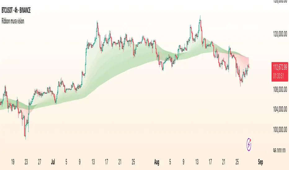
ATR RopeATR Rope is inspired by DonovanWall's "Range Filter". It implements a similar concept of filtering out smaller market movements and adjusting only for larger moves. In addition, this indicator goes one step deeper by producing actionable zones to determine market state. (Trend vs. Consolidation)
> Background
When reading up on the Range Filter indicator, it reminded me exactly of a Rope stabilization drawing tool in a program I use frequently. Rope stabilization essentially attaches a fixed length "rope" to your cursor and an anchor point (Brush). As you move your cursor, you are pulling the brush behind it. The cursor (of course) will not pull the brush until the rope is fully extended, this behavior filters out jittery movements and is used to produce smoother drawing curves.
If compared visually side-by-side, you will notice that this indicator bears striking resemblance to its inspiration.
> Goal
Other than simply distinguishing price movements between meaningful and noise, this indicator strives to create a rigid structure to frame market movements and lack-there-of, such as when to anticipate trend, and when to suspect consolidation.
Since the indicator works based on an ATR range, the resulting ATR Channel does well to get reactions from price at its extremes. Naturally, when consolidating, price will remain within the channel, neither pushing the channel significantly up or down. Likewise, when trending, price will continue to push the channel in a single direction.
With the goal of keeping it quick and simple, this indicator does not do any smoothing of data feeds, and is simply based on the deviation of price from the central rope. Adjusting the rope when price extends past the threshold created by +/- ATR from the rope.
> Features & Behaviors
- ATR Rope
ATR Rope is displayed as a 3 color single line.
This can be considered the center line, or the directional line, whichever you'd prefer.
The main point of the Rope display is to indicate direction, however it also is factually the center of the current working range.
- ATR Rope Color
When the rope's value moves up, it changes to green (uptrend), when down, red (downtrend).
When the source crosses the rope, it turns blue (flat).
With these simple rules, we've formed a structure to view market movements.
- Consolidation Zones
Consolidation Zones generate from "Flat" areas, and extend into subsequent trend areas. Consolidation is simply areas where price has crossed the Rope and remains inside the range. Over these periods, the upper and lower values are accumulated and averaged together to form the "Consolidation Zone" values. These zones are draw live, so values are averaged as the flat areas progress and don't repaint, so all values seen historically are as they would appear live.
- ATR Channel
ATR Channel displays the upper and lower bounds of the working range.
When the source moves beyond this range, the rope is adjusted based on the distance from the source to the channel. This range can be extremely useful to view, but by default it is hidden.
> Application
This indicator is not created to provide signals, or serve as a "complete" system.
(People who didn't read this far will still comment for signals. :) )
This is created to be used alongside manual interpretation and intuition. This indicator is not meant to constrain any users into a box, and I would actually encourage an open mind and idea generation, as the application of this indicator can take various forms.
> Examples
As you would probably already know, price movement can be fast impulses, and movement can be slow bleeds. In the screenshot below, we are using movements from and to consolidation zones to classify weak trend and strong trend. As you can see, there are also areas of consolidation which get broken out of and confirmed for the larger moves.
Author's Note: In each of these examples, I have outlined the start and end of each session. These examples come from 1 Min Future charts, and have specifically been framed with day trading in mind.
"Breakout Retest" or "Support/Resistance Flips" or "Structure Retests" are all generally the same thing, with different traders referring to them by different names, all of which can be seen throughout these examples.
In the next example, we have a day which started with an early reversal leading into long, slow, trend. Notice how each area throughout the trend essentially moves slightly higher, then consolidates while holding support of the previous zone. This day had a few sharp movements, however there was a large amount of neutrality throughout this day with continuous higher lows.
In contrast to the previous example, next up, we have a very choppy day. Throughout which we see a significant amount of retests before fast directional movements. We also see a few examples of places where previous zones remained relevant into the future. While the zones only display into the resulting trend area, they do not become immediately meaningless once they stop drawing.
> Abstract
In the screenshot below, I have stacked 2 of these indicators, using the high as the source for one and the low as the source for the other. I've hidden lines of the high and low channels to create a 4 lined channel based on the wicks of price.
This is not necessary to use the indicator, but should help provide an idea of creative ways the simple indicator could be used to produce more complicated analysis.
If you've made it this far, I would hope it's clear to you how this indicator could provide value to your trading.
Thank you to DonovonWall for the inspiration.
Enjoy!

Triple StochasticTriple Stochastic Elasticity Indicator
This custom indicator leverages the power of multi-timeframe analysis by combining three Stochastic Oscillators across different timeframes to identify potential trade entries based on elasticity and divergence between momentum curves.
📊 How It Works:
The indicator plots Stochastic values from three timeframes (e.g., 5m, 15m, and 1h), allowing you to observe how momentum behaves at different scales.
It highlights moments of elasticity—where the Stochastics stretch apart and then begin to converge—potentially signaling a reversion opportunity or trend continuation.
By identifying these stretches and snapbacks in momentum alignment, you can better time your entries and exits with improved confidence.
🔍 Use Case:
Look for divergence or convergence between the Stochastics.
Ideal for trend-following entries, pullback setups, and momentum reversal spotting.
Works best when combined with price action, S/R zones, or volume confirmation.
🛠 Customization:
Timeframes for each Stochastic are fully customizable.
Options to tweak %K, %D, and smoothing values to fit your strategy.
I recommend to remove the D%
And set the following settings
5 : 3 : 3
14 : 3 : 3
56 : 12 :12
Visual alerts can be added for when certain conditions are met (e.g., all three Stochs cross overbought/oversold levels).

Vesica Piscis Visualization-Secret Geometry-AYNETExplanation
Customization Options:
circle_radius: Adjust the size of the circles.
line_color: Choose the color of the circles.
line_width: Adjust the thickness of the circle lines.
segments: Increase or decrease the smoothness of the circles (higher values make smoother circles but use more computational resources).
Placement:
The first circle is centered at circle1_x and the second is offset horizontally by 2 * circle_radius to ensure their centers intersect each other's circumference.
Intersection Highlight:
The intersection area is visually emphasized with a semi-transparent background (bgcolor), which can be customized or removed if unnecessary.
Smoothness:
The segments input determines how many points are used to create each circle. Higher values create smoother curves.
Adjustments
Ensure the circles fit within the visible chart area by adjusting circle1_x and circle_radius.
If needed, you can add additional features, such as drawing lines to connect the centers or labeling the Vesica Piscis region.
Let me know if you want further refinements or additional features!

Machine Learning Signal FilterIntroducing the "Machine Learning Signal Filter," an innovative trading indicator designed to leverage the power of machine learning to enhance trading strategies. This tool combines advanced data processing capabilities with user-friendly customization options, offering traders a sophisticated yet accessible means to optimize their market analysis and decision-making processes. Importantly, this indicator does not repaint, ensuring that signals remain consistent and reliable after they are generated.
Machine Learning Integration
The "Machine Learning Signal Filter" employs machine learning algorithms to analyze historical price data and identify patterns that may not be immediately apparent through traditional technical analysis. By utilizing techniques such as regression analysis and neural networks, the indicator continuously learns from new data, refining its predictive capabilities over time. This dynamic adaptability allows the indicator to adjust to changing market conditions, potentially improving the accuracy of trading signals.
Key Features and Benefits
Dynamic Signal Generation: The indicator uses machine learning to generate buy and sell signals based on complex data patterns. This approach enables it to adapt to evolving market trends, offering traders timely and relevant insights. Crucially, the indicator does not repaint, providing reliable signals that traders can trust.
Customizable Parameters: Users can fine-tune the indicator to suit their specific trading styles by adjusting settings such as the temporal synchronization and neural pulse rate. This flexibility ensures that the indicator can be tailored to different market environments.
Visual Clarity and Usability: The indicator provides clear visual cues on the chart, including color-coded signals and optional display of signal curves. Users can also customize the table's position and text size, enhancing readability and ease of use.
Comprehensive Performance Metrics: The indicator includes a detailed metrics table that displays key performance indicators such as return rates, trade counts, and win/loss ratios. This feature helps traders assess the effectiveness of their strategies and make data-driven decisions.
How It Works
The core of the "Machine Learning Signal Filter" is its ability to process and learn from large datasets. By applying machine learning models, the indicator identifies potential trading opportunities based on historical data patterns. It uses regression techniques to predict future price movements and neural networks to enhance pattern recognition. As new data is introduced, the indicator refines its algorithms, improving its accuracy and reliability over time.
Use Cases
Trend Following: Ideal for traders seeking to capitalize on market trends, the indicator helps identify the direction and strength of price movements.
Scalping: With its ability to provide quick signals, the indicator is suitable for scalpers aiming for rapid profits in volatile markets.
Risk Management: By offering insights into trade performance, the indicator aids in managing risk and optimizing trade setups.
In summary, the "Machine Learning Signal Filter" is a powerful tool that combines the analytical strength of machine learning with the practical needs of traders. Its ability to adapt and provide actionable insights makes it an invaluable asset for navigating the complexities of financial markets.
The "Machine Learning Signal Filter" is a tool designed to assist traders by providing insights based on historical data and machine learning techniques. It does not guarantee profitable trades and should be used as part of a comprehensive trading strategy. Users are encouraged to conduct their own research and consider their financial situation before making trading decisions. Trading involves significant risk, and it is possible to lose more than the initial investment. Always trade responsibly and be aware of the risks involved.

Many Moving AveragesA smooth looking indicator created from a mix of ALMA and LRC curves. Includes alternative calculation for both which I came up with through trial and error so a variety of combinations work to varying degrees. Just something I was playing around with that looked pretty nice in the end.
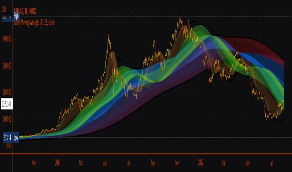
Excellent ADXThe Average Directional movement indeX (ADX) is an indicator that helps you determine the trend direction, pivot points, and much more else! But it looks not so easy as other famous indicators. It seems strange or even terrible, but don't be afraid. Let's understand how it works and get its power into your analysis tactics.
In the beginning, imagine a drunk man goes through a ladder: step by step. Up, up, down, up, down, down, up...
How can we understand which direction he goes? Exactly! We can count the number of steps in each direction. In the above example, in the upward – 4, in the downward – 3. So, it looks like he goes in an upward direction.
The ADX indicator counts the same steps, but for price. The size of each step equals 1 ATR for "DI Length" candles. On the indicator chart, we have the green and red lines. The green line represents a number of steps upward. The red line shows one downward. When the red line upper green, then the price goes below, then the trend is directed down. Later the green line comes above the red one, and then the trend changes the direction to upward. Wow? After that, you can easy detect the trend direction on the market!
But it is still not the end. On the chart, we also have the fat blue line. This is the ADX line, and it represents the power of the trend. It is calculated from a distance between the green and red curves. The ADX line value grows if the distance is increased. If the movement is really powerful, then a number of steps into a direction much more prominent than one in an opposed direction. Then the blue line grows faster. But if the growth has stopped and the blue line turns back or already had changed self-direction, then it is a signal that the trend has ended too. It's an excellent sign to close the position (but not always). Easy? Not quite. Thresholds help you there. The indicator has two additional parameters: upper and lower thresholds to evaluate the trend-over signal strength. An u-turn of the ADX line above the upper threshold sends a strong signal. If one occurs between both thresholds, it is a bit weak signal. But if the blue line goes below the lower threshold, it looks like there is no trend, and the price goes side. We can also say that the price goes side when the ADX value gradually falls down.
The Excellent ADX indicator helps you catch pivot/pullback signals based on green, red, and blue lines. Each such signal is highlighted as a green (buy) or red (sell) dot on the plot. The size of the dot represents the strength of the signal. You can also check the position of green and red lines from each other to determine the trend direction and the place where it has been changed. The Excellent ADX indicator helps you there too. It highlights the trend direction by the background-color, so you'll never miss it! The Excellent ADX good compliance with the Price Channel indicator built for the same length. You can use them together to be on a trend wave always!
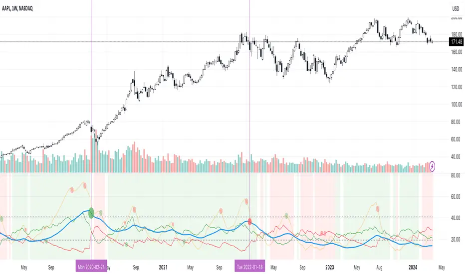
MACD ProMoving average convergence divergence pro.
Original MACD with new features, Including...
1. Three different modes.
Basic, Logarithmic, Percent (calculates difference of oscillator MAs in percent)
2. Additional moving averages for oscillator, signal and even histogram.
EMA, WMA (linearly weighted), LMA (logarithmically weighted), SMA
Volume Weighted RMA (I've been suggested to make a MACD with the VWEMA that I published recently but that was too fast, this almost 2 times slower because of using RMA instead of EMA)
VWRMA(s) (an alternative for VWRMA which uses candle formation to simulate the volume, can be useful when volume is not provided for the symbol or it is not proper)
And DEMA (Double Exponential MA)
3. Signal Displacement.
If you want to add some delay to signal, could help for extra confirmation of center crosses and removal of some falss ones.
4. Histogram Smoother.
For those who like the smooth curves. Can deliver a cleaner histogram even in volatile markets.
5. Bar color for more fun.

MAX TRENDS Spark 0.3.1.1This is a solid modification of Waves with extra volatility curves.
Very sophisticated for the day trading and forex swing.
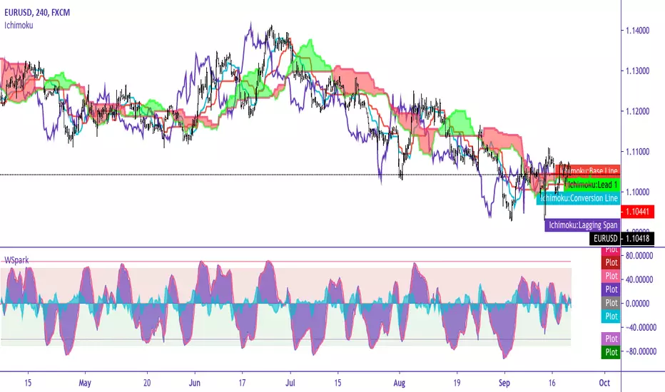
XBT Contango Calculator v1.1
This indicator measures value of basis (or spread) of current Futures contracts compared to spot. The default settings are specifically for Bitmex XBTU19 and XBTZ19 futures contracts. These will need to be updated after expiration. Also, it seems that Tradingview does not keep charts of expired contracts. If anyone knows how to import data from previous expired contracts, please let me know. This historical data could be valuable for evaluating previous XBT futures curves.
Also, VERY important to understand is this indicator only works with Spot Bitcoin charts (XBTUSD, BTCUSD, etc). If you add this to any other asset chart, it would not be useful (unless you changed settings to evaluate a different Futures product).
Contango and Backwardation are important fundamental indicators to keep track of while trading Futures markets. For a better explanation, Ugly Old Goat had done several medium articles on this. Please check out link below for his latest article on the subject...
uglyoldgoat.com
Notes on chart above should explain most of what you need to know on to use this indicator. The zero line is the spot price on the chart, so a positive value means Futures are trading at a premium (or in Contango). You can set a value of extreme Contango which will give an alert as red background (default setting is +$500). Green background will appear when Futures are trading at a discount to spot (Backwardation).
Hope some people get some use out of this. This is my first attempt at coding anything, so any feedback would be greatly appreciated!
BTC Donations: 3CypEdvBcvVHbqzHUt1FDiUG53U7pYWviV
Moving AverageDisplay of simple moving average and exponential mobile average depending on period.
Simple moving average are for D, W, and M period.
Minutes and Hours periods display exponential curves.