Enhanced Neowave Wave 1 Finder with ZigZagThis script is an advanced technical analysis indicator for the TradingView platform, written in Pine Script version 5. Its primary goal is to identify potential Elliott Wave "Wave 1" patterns, enhanced with principles from Neowave theory and a custom ZigZag indicator for more accurate pivot detection. The script is designed to be overlaid on the main price chart.
Core Functionality: Blending ZigZag and Neowave
The indicator's methodology is a two-part process. First, it identifies significant price swings using a robust ZigZag indicator. Then, it analyzes these swings based on a set of rules derived from Neowave and classic technical analysis to validate them as potential Wave 1 patterns.
Part 1: ZigZag Integration
The first major component is a comprehensive ZigZag indicator that forms the foundation for all subsequent analysis.
Pivot Detection: The pivots() function is the engine of the ZigZag. It scans the historical price data for significant high and low points (pivots) over a user-defined Length.
Segment Drawing: Once pivots are identified, the script draws lines connecting them, creating the classic ZigZag pattern on the chart.
Extended Direction & Ratios: This is an enhanced feature. The script doesn't just identify highs and lows; it categorizes them as:
Higher High (HH) or Lower High (LH)
Lower Low (LL) or Higher Low (HL)
This classification is crucial for understanding the market structure. It also calculates the price ratio of the most recent ZigZag leg relative to the previous one, which is used later for pattern validation.
Dynamic Updates: The ZigZag is not static. On each new bar, it can update its most recent pivot point if a new, more extreme price (a higher high or a lower low) is printed before the direction officially changes. This ensures the ZigZag is always reflecting the most current and significant price action.
Part 2: Neowave Wave 1 Finder
With the market structure defined by the ZigZag, the second part of the script applies a rigorous set of rules to identify potential Wave 1 patterns. A Wave 1 is the initial move of a new trend in Elliott Wave theory.
Key Validation Criteria
For a price move between two ZigZag pivots to be considered a valid Wave 1, it must pass a series of checks:
Significance: The move must have a minimum percentage change (Minimum Wave Length) and last for a minimum number of bars, filtering out insignificant noise.
Volume Confirmation: A genuine impulse wave is typically supported by increasing volume. The script checks if the volume during the potential Wave 1 is significantly higher than the recent average (Volume Increase Threshold).
Momentum Alignment: The direction of the wave must be confirmed by momentum indicators.
For a bullish (upward) Wave 1, the Relative Strength Index (RSI) must be in a bullish regime (above 50) and the MACD line must be above its signal line.
For a bearish (downward) Wave 1, the RSI must be below 50 and the MACD line must be below its signal line.
Structural Analysis (Impulse vs. Diagonal): The script attempts to differentiate between two types of Wave 1:
Impulse Wave: A strong, clean, and direct move.
Diagonal Wave: A more complex, overlapping, and often wedge-shaped pattern. This is identified by analyzing the time and price complexity of the move, along with the ZigZag leg ratios.
Wave 2 Retracement Check: A critical Neowave rule is that a valid Wave 1 must be followed by a valid Wave 2 retracement. The script looks at the next ZigZag leg to ensure it doesn't retrace more than 100% of the potential Wave 1. It also uses the ZigZag ratios to confirm the retracement falls within typical Fibonacci levels (e.g., 38.2% to 78.6%).
Display and User Interface
The script provides a rich visual experience to aid the trader in their analysis.
Wave Labels and Boxes: When a valid Wave 1 is detected, it is highlighted with a colored line (green for bullish, red for bearish) and a shaded background box. A label clearly marks it as "Wave 1 IMPULSE" or "Wave 1 DIAGONAL".
Fibonacci Retracement Levels: Upon detection of a Wave 1, the script automatically draws key Fibonacci retracement levels (38.2%, 50%, 61.8%, 78.6%). These levels are potential targets for the end of the subsequent Wave 2, offering potential entry points for a Wave 3 trade.
Information Labels: Additional labels provide at-a-glance confirmation of the conditions, showing whether volume and momentum criteria were met.
Customizable Inputs: Users have extensive control over the indicator's parameters, including the ZigZag length, volume thresholds, RSI levels, and the colors of all visual elements.
Alerts: The indicator can be configured to generate an alert whenever a new bullish or bearish Wave 1 pattern is confirmed, allowing traders to be notified of potential opportunities in real-time.
Wyszukaj w skryptach "Elliot"

Golden Pocket Syndicate [GPS]Golden Pocket Syndicate is a multi-layered market analysis toolkit built for precision entries and sniper-style reversals in both trending and ranging conditions. The script fuses volume dynamics, golden pocket structures, market maker behavior, and liquidation cluster tracking into one high-confluence system.
Core Features:
• 📐 Golden Pocket Zones: Dynamic GP levels from daily, weekly, monthly, and yearly timeframes. These levels update in real-time and serve as confluence zones for entries and exits.
• 📊 WaveTrend Divergence Diamonds: Momentum shifts are detected using a custom filtered WaveTrend cross system to mark high-probability reversal conditions.
• 🧠 Market Maker Premium Divergence: Tracks price dislocation between CME and Binance to detect large player manipulation using a configurable premium threshold.
• 💎 MM Reversal Diamonds: Identifies potential market maker traps and large player pivots using historical candle behavior, EMA alignment, and price structure breaks.
• 📉 Stealth Liquidation Cluster Arrows: Volume-based liquidation pressure visualized as lightweight directional arrows based on calculated wick expansion and volume bursts. Highlights key zones where price is likely to bounce or reject.
• 🧭 Trend Validation: Uses volume-based trend conditions and short-term EMA positioning to further qualify signals and eliminate noise.
How to Use:
This indicator is designed to help traders visualize confluence between key institutional price levels, momentum shifts, and volume-based pressure points. Long/short opportunities can be explored at marked reversal diamonds or liquidation zones that align with key GP levels. Intended for use on higher timeframes (15m to 4H), though flexible across any pair or market.

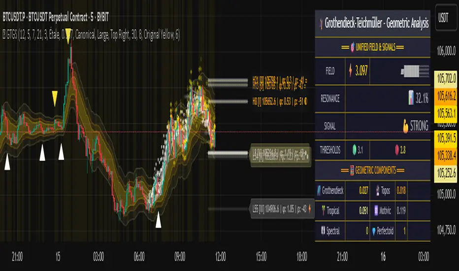
Grothendieck-Teichmüller Geometric SynthesisDskyz's Grothendieck-Teichmüller Geometric Synthesis (GTGS)
THEORETICAL FOUNDATION: A SYMPHONY OF GEOMETRIES
The 🎓 GTGS is built upon a revolutionary premise: that market dynamics can be modeled as geometric and topological structures. While not a literal academic implementation—such a task would demand computational power far beyond current trading platforms—it leverages core ideas from advanced mathematical theories as powerful analogies and frameworks for its algorithms. Each component translates an abstract concept into a practical market calculation, distinguishing GTGS by identifying deeper structural patterns rather than relying on standard statistical measures.
1. Grothendieck-Teichmüller Theory: Deforming Market Structure
The Theory : Studies symmetries and deformations of geometric objects, focusing on the "absolute" structure of mathematical spaces.
Indicator Analogy : The calculate_grothendieck_field function models price action as a "deformation" from its immediate state. Using the nth root of price ratios (math.pow(price_ratio, 1.0/prime)), it measures market "shape" stretching or compression, revealing underlying tensions and potential shifts.
2. Topos Theory & Sheaf Cohomology: From Local to Global Patterns
The Theory : A framework for assembling local properties into a global picture, with cohomology measuring "obstructions" to consistency.
Indicator Analogy : The calculate_topos_coherence function uses sine waves (math.sin) to represent local price "sections." Summing these yields a "cohomology" value, quantifying price action consistency. High values indicate coherent trends; low values signal conflict and uncertainty.
3. Tropical Geometry: Simplifying Complexity
The Theory : Transforms complex multiplicative problems into simpler, additive, piecewise-linear ones using min(a, b) for addition and a + b for multiplication.
Indicator Analogy : The calculate_tropical_metric function applies tropical_add(a, b) => math.min(a, b) to identify the "lowest energy" state among recent price points, pinpointing critical support levels non-linearly.
4. Motivic Cohomology & Non-Commutative Geometry
The Theory : Studies deep arithmetic and quantum-like properties of geometric spaces.
Indicator Analogy : The motivic_rank and spectral_triple functions compute weighted sums of historical prices to capture market "arithmetic complexity" and "spectral signature." Higher values reflect structured, harmonic price movements.
5. Perfectoid Spaces & Homotopy Type Theory
The Theory : Abstract fields dealing with p-adic numbers and logical foundations of mathematics.
Indicator Analogy : The perfectoid_conv and type_coherence functions analyze price convergence and path identity, assessing the "fractal dust" of price differences and price path cohesion, adding fractal and logical analysis.
The Combination is Key : No single theory dominates. GTGS ’s Unified Field synthesizes all seven perspectives into a comprehensive score, ensuring signals reflect deep structural alignment across mathematical domains.
🎛️ INPUTS: CONFIGURING THE GEOMETRIC ENGINE
The GTGS offers a suite of customizable inputs, allowing traders to tailor its behavior to specific timeframes, market sectors, and trading styles. Below is a detailed breakdown of key input groups, their functionality, and optimization strategies, leveraging provided tooltips for precision.
Grothendieck-Teichmüller Theory Inputs
🧬 Deformation Depth (Absolute Galois) :
What It Is : Controls the depth of Galois group deformations analyzed in market structure.
How It Works : Measures price action deformations under automorphisms of the absolute Galois group, capturing market symmetries.
Optimization :
Higher Values (15-20) : Captures deeper symmetries, ideal for major trends in swing trading (4H-1D).
Lower Values (3-8) : Responsive to local deformations, suited for scalping (1-5min).
Timeframes :
Scalping (1-5min) : 3-6 for quick local shifts.
Day Trading (15min-1H) : 8-12 for balanced analysis.
Swing Trading (4H-1D) : 12-20 for deep structural trends.
Sectors :
Stocks : Use 8-12 for stable trends.
Crypto : 3-8 for volatile, short-term moves.
Forex : 12-15 for smooth, cyclical patterns.
Pro Tip : Increase in trending markets to filter noise; decrease in choppy markets for sensitivity.
🗼 Teichmüller Tower Height :
What It Is : Determines the height of the Teichmüller modular tower for hierarchical pattern detection.
How It Works : Builds modular levels to identify nested market patterns.
Optimization :
Higher Values (6-8) : Detects complex fractals, ideal for swing trading.
Lower Values (2-4) : Focuses on primary patterns, faster for scalping.
Timeframes :
Scalping : 2-3 for speed.
Day Trading : 4-5 for balanced patterns.
Swing Trading : 5-8 for deep fractals.
Sectors :
Indices : 5-8 for robust, long-term patterns.
Crypto : 2-4 for rapid shifts.
Commodities : 4-6 for cyclical trends.
Pro Tip : Higher towers reveal hidden fractals but may slow computation; adjust based on hardware.
🔢 Galois Prime Base :
What It Is : Sets the prime base for Galois field computations.
How It Works : Defines the field extension characteristic for market analysis.
Optimization :
Prime Characteristics :
2 : Binary markets (up/down).
3 : Ternary states (bull/bear/neutral).
5 : Pentagonal symmetry (Elliott waves).
7 : Heptagonal cycles (weekly patterns).
11,13,17,19 : Higher-order patterns.
Timeframes :
Scalping/Day Trading : 2 or 3 for simplicity.
Swing Trading : 5 or 7 for wave or cycle detection.
Sectors :
Forex : 5 for Elliott wave alignment.
Stocks : 7 for weekly cycle consistency.
Crypto : 3 for volatile state shifts.
Pro Tip : Use 7 for most markets; 5 for Elliott wave traders.
Topos Theory & Sheaf Cohomology Inputs
🏛️ Temporal Site Size :
What It Is : Defines the number of time points in the topological site.
How It Works : Sets the local neighborhood for sheaf computations, affecting cohomology smoothness.
Optimization :
Higher Values (30-50) : Smoother cohomology, better for trends in swing trading.
Lower Values (5-15) : Responsive, ideal for reversals in scalping.
Timeframes :
Scalping : 5-10 for quick responses.
Day Trading : 15-25 for balanced analysis.
Swing Trading : 25-50 for smooth trends.
Sectors :
Stocks : 25-35 for stable trends.
Crypto : 5-15 for volatility.
Forex : 20-30 for smooth cycles.
Pro Tip : Match site size to your average holding period in bars for optimal coherence.
📐 Sheaf Cohomology Degree :
What It Is : Sets the maximum degree of cohomology groups computed.
How It Works : Higher degrees capture complex topological obstructions.
Optimization :
Degree Meanings :
1 : Simple obstructions (basic support/resistance).
2 : Cohomological pairs (double tops/bottoms).
3 : Triple intersections (complex patterns).
4-5 : Higher-order structures (rare events).
Timeframes :
Scalping/Day Trading : 1-2 for simplicity.
Swing Trading : 3 for complex patterns.
Sectors :
Indices : 2-3 for robust patterns.
Crypto : 1-2 for rapid shifts.
Commodities : 3-4 for cyclical events.
Pro Tip : Degree 3 is optimal for most trading; higher degrees for research or rare event detection.
🌐 Grothendieck Topology :
What It Is : Chooses the Grothendieck topology for the site.
How It Works : Affects how local data integrates into global patterns.
Optimization :
Topology Characteristics :
Étale : Finest topology, captures local-global principles.
Nisnevich : A1-invariant, good for trends.
Zariski : Coarse but robust, filters noise.
Fpqc : Faithfully flat, highly sensitive.
Sectors :
Stocks : Zariski for stability.
Crypto : Étale for sensitivity.
Forex : Nisnevich for smooth trends.
Indices : Zariski for robustness.
Timeframes :
Scalping : Étale for precision.
Swing Trading : Nisnevich or Zariski for reliability.
Pro Tip : Start with Étale for precision; switch to Zariski in noisy markets.
Unified Field Configuration Inputs
⚛️ Field Coupling Constant :
What It Is : Sets the interaction strength between geometric components.
How It Works : Controls signal amplification in the unified field equation.
Optimization :
Higher Values (0.5-1.0) : Strong coupling, amplified signals for ranging markets.
Lower Values (0.001-0.1) : Subtle signals for trending markets.
Timeframes :
Scalping : 0.5-0.8 for quick, strong signals.
Swing Trading : 0.1-0.3 for trend confirmation.
Sectors :
Crypto : 0.5-1.0 for volatility.
Stocks : 0.1-0.3 for stability.
Forex : 0.3-0.5 for balance.
Pro Tip : Default 0.137 (fine structure constant) is a balanced starting point; adjust up in choppy markets.
📐 Geometric Weighting Scheme :
What It Is : Determines the framework for combining geometric components.
How It Works : Adjusts emphasis on different mathematical structures.
Optimization :
Scheme Characteristics :
Canonical : Equal weighting, balanced.
Derived : Emphasizes higher-order structures.
Motivic : Prioritizes arithmetic properties.
Spectral : Focuses on frequency domain.
Sectors :
Stocks : Canonical for balance.
Crypto : Spectral for volatility.
Forex : Derived for structured moves.
Indices : Motivic for arithmetic cycles.
Timeframes :
Day Trading : Canonical or Derived for flexibility.
Swing Trading : Motivic for long-term cycles.
Pro Tip : Start with Canonical; experiment with Spectral in volatile markets.
Dashboard and Visual Configuration Inputs
📋 Show Enhanced Dashboard, 📏 Size, 📍 Position :
What They Are : Control dashboard visibility, size, and placement.
How They Work : Display key metrics like Unified Field , Resonance , and Signal Quality .
Optimization :
Scalping : Small size, Bottom Right for minimal chart obstruction.
Swing Trading : Large size, Top Right for detailed analysis.
Sectors : Universal across markets; adjust size based on screen setup.
Pro Tip : Use Large for analysis, Small for live trading.
📐 Show Motivic Cohomology Bands, 🌊 Morphism Flow, 🔮 Future Projection, 🔷 Holographic Mesh, ⚛️ Spectral Flow :
What They Are : Toggle visual elements representing mathematical calculations.
How They Work : Provide intuitive representations of market dynamics.
Optimization :
Timeframes :
Scalping : Enable Morphism Flow and Spectral Flow for momentum.
Swing Trading : Enable all for comprehensive analysis.
Sectors :
Crypto : Emphasize Morphism Flow and Future Projection for volatility.
Stocks : Focus on Cohomology Bands for stable trends.
Pro Tip : Disable non-essential visuals in fast markets to reduce clutter.
🌫️ Field Transparency, 🔄 Web Recursion Depth, 🎨 Mesh Color Scheme :
What They Are : Adjust visual clarity, complexity, and color.
How They Work : Enhance interpretability of visual elements.
Optimization :
Transparency : 30-50 for balanced visibility; lower for analysis.
Recursion Depth : 6-8 for balanced detail; lower for older hardware.
Color Scheme :
Purple/Blue : Analytical focus.
Green/Orange : Trading momentum.
Pro Tip : Use Neon Purple for deep analysis; Neon Green for active trading.
⏱️ Minimum Bars Between Signals :
What It Is : Minimum number of bars required between consecutive signals.
How It Works : Prevents signal clustering by enforcing a cooldown period.
Optimization :
Higher Values (10-20) : Fewer signals, avoids whipsaws, suited for swing trading.
Lower Values (0-5) : More responsive, allows quick reversals, ideal for scalping.
Timeframes :
Scalping : 0-2 bars for rapid signals.
Day Trading : 3-5 bars for balance.
Swing Trading : 5-10 bars for stability.
Sectors :
Crypto : 0-3 for volatility.
Stocks : 5-10 for trend clarity.
Forex : 3-7 for cyclical moves.
Pro Tip : Increase in choppy markets to filter noise.
Hardcoded Parameters
Tropical, Motivic, Spectral, Perfectoid, Homotopy Inputs : Fixed to optimize performance but influence calculations (e.g., tropical_degree=4 for support levels, perfectoid_prime=5 for convergence).
Optimization : Experiment with codebase modifications if advanced customization is needed, but defaults are robust across markets.
🎨 ADVANCED VISUAL SYSTEM: TRADING IN A GEOMETRIC UNIVERSE
The GTTMTSF ’s visuals are direct representations of its mathematics, designed for intuitive and precise trading decisions.
Motivic Cohomology Bands :
What They Are : Dynamic bands ( H⁰ , H¹ , H² ) representing cohomological support/resistance.
Color & Meaning : Colors reflect energy levels ( H⁰ tightest, H² widest). Breaks into H¹ signal momentum; H² touches suggest reversals.
How to Trade : Use for stop-loss/profit-taking. Band bounces with Dashboard confirmation are high-probability setups.
Morphism Flow (Webbing) :
What It Is : White particle streams visualizing market momentum.
Interpretation : Dense flows indicate strong trends; sparse flows signal consolidation.
How to Trade : Follow dominant flow direction; new flows post-consolidation signal trend starts.
Future Projection Web (Fractal Grid) :
What It Is : Fibonacci-period fractal projections of support/resistance.
Color & Meaning : Three-layer lines (white shadow, glow, colored quantum) with labels showing price, topological class, anomaly strength (φ), resonance (ρ), and obstruction ( H¹ ). ⚡ marks extreme anomalies.
How to Trade : Target ⚡/● levels for entries/exits. High-anomaly levels with weakening Unified Field are reversal setups.
Holographic Mesh & Spectral Flow :
What They Are : Visuals of harmonic interference and spectral energy.
How to Trade : Bright mesh nodes or strong Spectral Flow warn of building pressure before price movement.
📊 THE GEOMETRIC DASHBOARD: YOUR MISSION CONTROL
The Dashboard translates complex mathematics into actionable intelligence.
Unified Field & Signals :
FIELD : Master value (-10 to +10), synthesizing all geometric components. Extreme readings (>5 or <-5) signal structural limits, often preceding reversals or continuations.
RESONANCE : Measures harmony between geometric field and price-volume momentum. Positive amplifies bullish moves; negative amplifies bearish moves.
SIGNAL QUALITY : Confidence meter rating alignment. Trade only STRONG or EXCEPTIONAL signals for high-probability setups.
Geometric Components :
What They Are : Breakdown of seven mathematical engines.
How to Use : Watch for convergence. A strong Unified Field is reliable when components (e.g., Grothendieck , Topos , Motivic ) align. Divergence warns of trend weakening.
Signal Performance :
What It Is : Tracks indicator signal performance.
How to Use : Assesses real-time performance to build confidence and understand system behavior.
🚀 DEVELOPMENT & UNIQUENESS: BEYOND CONVENTIONAL ANALYSIS
The GTTMTSF was developed to analyze markets as evolving geometric objects, not statistical time-series.
Why This Is Unlike Anything Else :
Theoretical Depth : Uses geometry and topology, identifying patterns invisible to statistical tools.
Holistic Synthesis : Integrates seven deep mathematical frameworks into a cohesive Unified Field .
Creative Implementation : Translates PhD-level mathematics into functional Pine Script , blending theory and practice.
Immersive Visualization : Transforms charts into dynamic geometric landscapes for intuitive market understanding.
The GTTMTSF is more than an indicator; it’s a new lens for viewing markets, for traders seeking deeper insight into hidden order within chaos.
" Where there is matter, there is geometry. " - Johannes Kepler
— Dskyz , Trade with insight. Trade with anticipation.
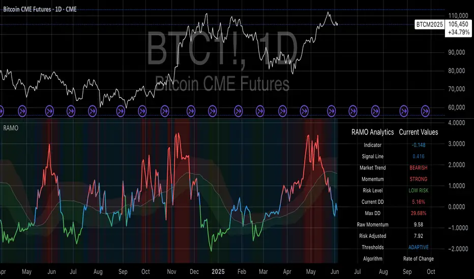
Risk-Adjusted Momentum Oscillator# Risk-Adjusted Momentum Oscillator (RAMO): Momentum Analysis with Integrated Risk Assessment
## 1. Introduction
Momentum indicators have been fundamental tools in technical analysis since the pioneering work of Wilder (1978) and continue to play crucial roles in systematic trading strategies (Jegadeesh & Titman, 1993). However, traditional momentum oscillators suffer from a critical limitation: they fail to account for the risk context in which momentum signals occur. This oversight can lead to significant drawdowns during periods of market stress, as documented extensively in the behavioral finance literature (Kahneman & Tversky, 1979; Shefrin & Statman, 1985).
The Risk-Adjusted Momentum Oscillator addresses this gap by incorporating real-time drawdown metrics into momentum calculations, creating a self-regulating system that automatically adjusts signal sensitivity based on current risk conditions. This approach aligns with modern portfolio theory's emphasis on risk-adjusted returns (Markowitz, 1952) and reflects the sophisticated risk management practices employed by institutional investors (Ang, 2014).
## 2. Theoretical Foundation
### 2.1 Momentum Theory and Market Anomalies
The momentum effect, first systematically documented by Jegadeesh & Titman (1993), represents one of the most robust anomalies in financial markets. Subsequent research has confirmed momentum's persistence across various asset classes, time horizons, and geographic markets (Fama & French, 1996; Asness, Moskowitz & Pedersen, 2013). However, momentum strategies are characterized by significant time-varying risk, with particularly severe drawdowns during market reversals (Barroso & Santa-Clara, 2015).
### 2.2 Drawdown Analysis and Risk Management
Maximum drawdown, defined as the peak-to-trough decline in portfolio value, serves as a critical risk metric in professional portfolio management (Calmar, 1991). Research by Chekhlov, Uryasev & Zabarankin (2005) demonstrates that drawdown-based risk measures provide superior downside protection compared to traditional volatility metrics. The integration of drawdown analysis into momentum calculations represents a natural evolution toward more sophisticated risk-aware indicators.
### 2.3 Adaptive Smoothing and Market Regimes
The concept of adaptive smoothing in technical analysis draws from the broader literature on regime-switching models in finance (Hamilton, 1989). Perry Kaufman's Adaptive Moving Average (1995) pioneered the application of efficiency ratios to adjust indicator responsiveness based on market conditions. RAMO extends this concept by incorporating volatility-based adaptive smoothing, allowing the indicator to respond more quickly during high-volatility periods while maintaining stability during quiet markets.
## 3. Methodology
### 3.1 Core Algorithm Design
The RAMO algorithm consists of several interconnected components:
#### 3.1.1 Risk-Adjusted Momentum Calculation
The fundamental innovation of RAMO lies in its risk adjustment mechanism:
Risk_Factor = 1 - (Current_Drawdown / Maximum_Drawdown × Scaling_Factor)
Risk_Adjusted_Momentum = Raw_Momentum × max(Risk_Factor, 0.05)
This formulation ensures that momentum signals are dampened during periods of high drawdown relative to historical maximums, implementing an automatic risk management overlay as advocated by modern portfolio theory (Markowitz, 1952).
#### 3.1.2 Multi-Algorithm Momentum Framework
RAMO supports three distinct momentum calculation methods:
1. Rate of Change: Traditional percentage-based momentum (Pring, 2002)
2. Price Momentum: Absolute price differences
3. Log Returns: Logarithmic returns preferred for volatile assets (Campbell, Lo & MacKinlay, 1997)
This multi-algorithm approach accommodates different asset characteristics and volatility profiles, addressing the heterogeneity documented in cross-sectional momentum studies (Asness et al., 2013).
### 3.2 Leading Indicator Components
#### 3.2.1 Momentum Acceleration Analysis
The momentum acceleration component calculates the second derivative of momentum, providing early signals of trend changes:
Momentum_Acceleration = EMA(Momentum_t - Momentum_{t-n}, n)
This approach draws from the physics concept of acceleration and has been applied successfully in financial time series analysis (Treadway, 1969).
#### 3.2.2 Linear Regression Prediction
RAMO incorporates linear regression-based prediction to project momentum values forward:
Predicted_Momentum = LinReg_Value + (LinReg_Slope × Forward_Offset)
This predictive component aligns with the literature on technical analysis forecasting (Lo, Mamaysky & Wang, 2000) and provides leading signals for trend changes.
#### 3.2.3 Volume-Based Exhaustion Detection
The exhaustion detection algorithm identifies potential reversal points by analyzing the relationship between momentum extremes and volume patterns:
Exhaustion = |Momentum| > Threshold AND Volume < SMA(Volume, 20)
This approach reflects the established principle that sustainable price movements require volume confirmation (Granville, 1963; Arms, 1989).
### 3.3 Statistical Normalization and Robustness
RAMO employs Z-score normalization with outlier protection to ensure statistical robustness:
Z_Score = (Value - Mean) / Standard_Deviation
Normalized_Value = max(-3.5, min(3.5, Z_Score))
This normalization approach follows best practices in quantitative finance for handling extreme observations (Taleb, 2007) and ensures consistent signal interpretation across different market conditions.
### 3.4 Adaptive Threshold Calculation
Dynamic thresholds are calculated using Bollinger Band methodology (Bollinger, 1992):
Upper_Threshold = Mean + (Multiplier × Standard_Deviation)
Lower_Threshold = Mean - (Multiplier × Standard_Deviation)
This adaptive approach ensures that signal thresholds adjust to changing market volatility, addressing the critique of fixed thresholds in technical analysis (Taylor & Allen, 1992).
## 4. Implementation Details
### 4.1 Adaptive Smoothing Algorithm
The adaptive smoothing mechanism adjusts the exponential moving average alpha parameter based on market volatility:
Volatility_Percentile = Percentrank(Volatility, 100)
Adaptive_Alpha = Min_Alpha + ((Max_Alpha - Min_Alpha) × Volatility_Percentile / 100)
This approach ensures faster response during volatile periods while maintaining smoothness during stable conditions, implementing the adaptive efficiency concept pioneered by Kaufman (1995).
### 4.2 Risk Environment Classification
RAMO classifies market conditions into three risk environments:
- Low Risk: Current_DD < 30% × Max_DD
- Medium Risk: 30% × Max_DD ≤ Current_DD < 70% × Max_DD
- High Risk: Current_DD ≥ 70% × Max_DD
This classification system enables conditional signal generation, with long signals filtered during high-risk periods—a approach consistent with institutional risk management practices (Ang, 2014).
## 5. Signal Generation and Interpretation
### 5.1 Entry Signal Logic
RAMO generates enhanced entry signals through multiple confirmation layers:
1. Primary Signal: Crossover between indicator and signal line
2. Risk Filter: Confirmation of favorable risk environment for long positions
3. Leading Component: Early warning signals via acceleration analysis
4. Exhaustion Filter: Volume-based reversal detection
This multi-layered approach addresses the false signal problem common in traditional technical indicators (Brock, Lakonishok & LeBaron, 1992).
### 5.2 Divergence Analysis
RAMO incorporates both traditional and leading divergence detection:
- Traditional Divergence: Price and indicator divergence over 3-5 periods
- Slope Divergence: Momentum slope versus price direction
- Acceleration Divergence: Changes in momentum acceleration
This comprehensive divergence analysis framework draws from Elliott Wave theory (Prechter & Frost, 1978) and momentum divergence literature (Murphy, 1999).
## 6. Empirical Advantages and Applications
### 6.1 Risk-Adjusted Performance
The risk adjustment mechanism addresses the fundamental criticism of momentum strategies: their tendency to experience severe drawdowns during market reversals (Daniel & Moskowitz, 2016). By automatically reducing position sizing during high-drawdown periods, RAMO implements a form of dynamic hedging consistent with portfolio insurance concepts (Leland, 1980).
### 6.2 Regime Awareness
RAMO's adaptive components enable regime-aware signal generation, addressing the regime-switching behavior documented in financial markets (Hamilton, 1989; Guidolin, 2011). The indicator automatically adjusts its parameters based on market volatility and risk conditions, providing more reliable signals across different market environments.
### 6.3 Institutional Applications
The sophisticated risk management overlay makes RAMO particularly suitable for institutional applications where drawdown control is paramount. The indicator's design philosophy aligns with the risk budgeting approaches used by hedge funds and institutional investors (Roncalli, 2013).
## 7. Limitations and Future Research
### 7.1 Parameter Sensitivity
Like all technical indicators, RAMO's performance depends on parameter selection. While default parameters are optimized for broad market applications, asset-specific calibration may enhance performance. Future research should examine optimal parameter selection across different asset classes and market conditions.
### 7.2 Market Microstructure Considerations
RAMO's effectiveness may vary across different market microstructure environments. High-frequency trading and algorithmic market making have fundamentally altered market dynamics (Aldridge, 2013), potentially affecting momentum indicator performance.
### 7.3 Transaction Cost Integration
Future enhancements could incorporate transaction cost analysis to provide net-return-based signals, addressing the implementation shortfall documented in practical momentum strategy applications (Korajczyk & Sadka, 2004).
## References
Aldridge, I. (2013). *High-Frequency Trading: A Practical Guide to Algorithmic Strategies and Trading Systems*. 2nd ed. Hoboken, NJ: John Wiley & Sons.
Ang, A. (2014). *Asset Management: A Systematic Approach to Factor Investing*. New York: Oxford University Press.
Arms, R. W. (1989). *The Arms Index (TRIN): An Introduction to the Volume Analysis of Stock and Bond Markets*. Homewood, IL: Dow Jones-Irwin.
Asness, C. S., Moskowitz, T. J., & Pedersen, L. H. (2013). Value and momentum everywhere. *Journal of Finance*, 68(3), 929-985.
Barroso, P., & Santa-Clara, P. (2015). Momentum has its moments. *Journal of Financial Economics*, 116(1), 111-120.
Bollinger, J. (1992). *Bollinger on Bollinger Bands*. New York: McGraw-Hill.
Brock, W., Lakonishok, J., & LeBaron, B. (1992). Simple technical trading rules and the stochastic properties of stock returns. *Journal of Finance*, 47(5), 1731-1764.
Calmar, T. (1991). The Calmar ratio: A smoother tool. *Futures*, 20(1), 40.
Campbell, J. Y., Lo, A. W., & MacKinlay, A. C. (1997). *The Econometrics of Financial Markets*. Princeton, NJ: Princeton University Press.
Chekhlov, A., Uryasev, S., & Zabarankin, M. (2005). Drawdown measure in portfolio optimization. *International Journal of Theoretical and Applied Finance*, 8(1), 13-58.
Daniel, K., & Moskowitz, T. J. (2016). Momentum crashes. *Journal of Financial Economics*, 122(2), 221-247.
Fama, E. F., & French, K. R. (1996). Multifactor explanations of asset pricing anomalies. *Journal of Finance*, 51(1), 55-84.
Granville, J. E. (1963). *Granville's New Key to Stock Market Profits*. Englewood Cliffs, NJ: Prentice-Hall.
Guidolin, M. (2011). Markov switching models in empirical finance. In D. N. Drukker (Ed.), *Missing Data Methods: Time-Series Methods and Applications* (pp. 1-86). Bingley: Emerald Group Publishing.
Hamilton, J. D. (1989). A new approach to the economic analysis of nonstationary time series and the business cycle. *Econometrica*, 57(2), 357-384.
Jegadeesh, N., & Titman, S. (1993). Returns to buying winners and selling losers: Implications for stock market efficiency. *Journal of Finance*, 48(1), 65-91.
Kahneman, D., & Tversky, A. (1979). Prospect theory: An analysis of decision under risk. *Econometrica*, 47(2), 263-291.
Kaufman, P. J. (1995). *Smarter Trading: Improving Performance in Changing Markets*. New York: McGraw-Hill.
Korajczyk, R. A., & Sadka, R. (2004). Are momentum profits robust to trading costs? *Journal of Finance*, 59(3), 1039-1082.
Leland, H. E. (1980). Who should buy portfolio insurance? *Journal of Finance*, 35(2), 581-594.
Lo, A. W., Mamaysky, H., & Wang, J. (2000). Foundations of technical analysis: Computational algorithms, statistical inference, and empirical implementation. *Journal of Finance*, 55(4), 1705-1765.
Markowitz, H. (1952). Portfolio selection. *Journal of Finance*, 7(1), 77-91.
Murphy, J. J. (1999). *Technical Analysis of the Financial Markets: A Comprehensive Guide to Trading Methods and Applications*. New York: New York Institute of Finance.
Prechter, R. R., & Frost, A. J. (1978). *Elliott Wave Principle: Key to Market Behavior*. Gainesville, GA: New Classics Library.
Pring, M. J. (2002). *Technical Analysis Explained: The Successful Investor's Guide to Spotting Investment Trends and Turning Points*. 4th ed. New York: McGraw-Hill.
Roncalli, T. (2013). *Introduction to Risk Parity and Budgeting*. Boca Raton, FL: CRC Press.
Shefrin, H., & Statman, M. (1985). The disposition to sell winners too early and ride losers too long: Theory and evidence. *Journal of Finance*, 40(3), 777-790.
Taleb, N. N. (2007). *The Black Swan: The Impact of the Highly Improbable*. New York: Random House.
Taylor, M. P., & Allen, H. (1992). The use of technical analysis in the foreign exchange market. *Journal of International Money and Finance*, 11(3), 304-314.
Treadway, A. B. (1969). On rational entrepreneurial behavior and the demand for investment. *Review of Economic Studies*, 36(2), 227-239.
Wilder, J. W. (1978). *New Concepts in Technical Trading Systems*. Greensboro, NC: Trend Research.
Trend of Multiple Oscillator Dashboard ModifiedDescription: The "Trend of Multiple Oscillator Dashboard Modified" is a powerful Pine Script indicator that provides a dashboard view of various oscillator and trend-following indicators across multiple timeframes. This indicator helps traders to assess trend conditions comprehensively by integrating popular technical indicators, including MACD, EMA, Stochastic, Elliott Wave, DID (Curta, Media, Longa), Price Volume Trend (PVT), Kuskus Trend, and Wave Trend Oscillator. Each indicator’s trend signal (bullish, bearish, or neutral) is displayed in a color-coded dashboard, making it easy to spot the consensus or divergence in trends across different timeframes.
Key Features:
Multi-Timeframe Analysis: Displays trend signals across five predefined timeframes (1, 2, 3, 5, and 10 minutes) for each included indicator.
Customizable Inputs: Allows for customization of key parameters for each oscillator and trend-following indicator.
Trend Interpretation: Each indicator is visually represented with green (bullish), red (bearish), and yellow (neutral) trend markers, making trend identification intuitive and quick.
Trade Condition Controls: Input options for the number of positive and negative conditions needed to trigger entries and exits, allowing users to refine the decision-making criteria.
Delay Management: Options for re-entry conditions based on both price movement (in points) and the minimum number of candles since the last exit, giving users flexibility in managing trade entries.
Usage: This indicator is ideal for traders who rely on multiple oscillators and moving averages to gauge trend direction and strength across timeframes. The dashboard allows users to observe trends at a glance and make informed decisions based on the alignment of various trend indicators. It’s particularly useful in consolidating signals for strategies that require multiple conditions to align before entering or exiting trades.
Note: Ensure that you’re familiar with each oscillator’s functionality, as some indicators like Elliott Wave and Wave Trend are simplified for visual coherence in this dashboard.
Disclaimer: This script is intended for educational and informational purposes only. Use it with caution and adapt it to your specific trading plan.
Developer's Remark: "This indicator's comprehensive design allows traders to filter noise and identify the most robust trends effectively. Use it to visualize trends across timeframes, understand oscillator behavior, and enhance decision-making with a more strategic approach."

PubLibPatternLibrary "PubLibPattern"
pattern conditions for indicator and strategy development
bear_5_0(ab_low_tol, ab_up_tol, bc_low_tol, bc_up_tol, cd_low_tol, cd_up_tol)
bearish 5-0 harmonic pattern condition
Parameters:
ab_low_tol (float)
ab_up_tol (float)
bc_low_tol (float)
bc_up_tol (float)
cd_low_tol (float)
cd_up_tol (float)
Returns: bool
bull_5_0(ab_low_tol, ab_up_tol, bc_low_tol, bc_up_tol, cd_low_tol, cd_up_tol)
bullish 5-0 harmonic pattern condition
Parameters:
ab_low_tol (float)
ab_up_tol (float)
bc_low_tol (float)
bc_up_tol (float)
cd_low_tol (float)
cd_up_tol (float)
Returns: bool
bear_abcd(bc_low_tol, bc_up_tol, cd_low_tol, cd_up_tol)
bearish abcd harmonic pattern condition
Parameters:
bc_low_tol (float)
bc_up_tol (float)
cd_low_tol (float)
cd_up_tol (float)
Returns: bool
bull_abcd(bc_low_tol, bc_up_tol, cd_low_tol, cd_up_tol)
bullish abcd harmonic pattern condition
Parameters:
bc_low_tol (float)
bc_up_tol (float)
cd_low_tol (float)
cd_up_tol (float)
Returns: bool
bear_alt_bat(ab_low_tol, ab_up_tol, bc_low_tol, bc_up_tol, cd_low_tol, cd_up_tol, ad_low_tol, ad_up_tol)
bearish alternate bat harmonic pattern condition
Parameters:
ab_low_tol (float)
ab_up_tol (float)
bc_low_tol (float)
bc_up_tol (float)
cd_low_tol (float)
cd_up_tol (float)
ad_low_tol (float)
ad_up_tol (float)
Returns: bool
bull_alt_bat(ab_low_tol, ab_up_tol, bc_low_tol, bc_up_tol, cd_low_tol, cd_up_tol, ad_low_tol, ad_up_tol)
bullish alternate bat harmonic pattern condition
Parameters:
ab_low_tol (float)
ab_up_tol (float)
bc_low_tol (float)
bc_up_tol (float)
cd_low_tol (float)
cd_up_tol (float)
ad_low_tol (float)
ad_up_tol (float)
Returns: bool
bear_bat(ab_low_tol, ab_up_tol, bc_low_tol, bc_up_tol, cd_low_tol, cd_up_tol, ad_low_tol, ad_up_tol)
bearish bat harmonic pattern condition
Parameters:
ab_low_tol (float)
ab_up_tol (float)
bc_low_tol (float)
bc_up_tol (float)
cd_low_tol (float)
cd_up_tol (float)
ad_low_tol (float)
ad_up_tol (float)
Returns: bool
bull_bat(ab_low_tol, ab_up_tol, bc_low_tol, bc_up_tol, cd_low_tol, cd_up_tol, ad_low_tol, ad_up_tol)
bullish bat harmonic pattern condition
Parameters:
ab_low_tol (float)
ab_up_tol (float)
bc_low_tol (float)
bc_up_tol (float)
cd_low_tol (float)
cd_up_tol (float)
ad_low_tol (float)
ad_up_tol (float)
Returns: bool
bear_butterfly(ab_low_tol, ab_up_tol, bc_low_tol, bc_up_tol, cd_low_tol, cd_up_tol, ad_low_tol, ad_up_tol)
bearish butterfly harmonic pattern condition
Parameters:
ab_low_tol (float)
ab_up_tol (float)
bc_low_tol (float)
bc_up_tol (float)
cd_low_tol (float)
cd_up_tol (float)
ad_low_tol (float)
ad_up_tol (float)
Returns: bool
bull_butterfly(ab_low_tol, ab_up_tol, bc_low_tol, bc_up_tol, cd_low_tol, cd_up_tol, ad_low_tol, ad_up_tol)
bullish butterfly harmonic pattern condition
Parameters:
ab_low_tol (float)
ab_up_tol (float)
bc_low_tol (float)
bc_up_tol (float)
cd_low_tol (float)
cd_up_tol (float)
ad_low_tol (float)
ad_up_tol (float)
Returns: bool
bear_cassiopeia_a(ab_low_tol, ab_up_tol, bc_low_tol, bc_up_tol, cd_low_tol, cd_up_tol)
bearish cassiopeia a harmonic pattern condition
Parameters:
ab_low_tol (float)
ab_up_tol (float)
bc_low_tol (float)
bc_up_tol (float)
cd_low_tol (float)
cd_up_tol (float)
Returns: bool
bull_cassiopeia_a(ab_low_tol, ab_up_tol, bc_low_tol, bc_up_tol, cd_low_tol, cd_up_tol)
bullish cassiopeia a harmonic pattern condition
Parameters:
ab_low_tol (float)
ab_up_tol (float)
bc_low_tol (float)
bc_up_tol (float)
cd_low_tol (float)
cd_up_tol (float)
Returns: bool
bear_cassiopeia_b(ab_low_tol, ab_up_tol, bc_low_tol, bc_up_tol, cd_low_tol, cd_up_tol)
bearish cassiopeia b harmonic pattern condition
Parameters:
ab_low_tol (float)
ab_up_tol (float)
bc_low_tol (float)
bc_up_tol (float)
cd_low_tol (float)
cd_up_tol (float)
Returns: bool
bull_cassiopeia_b(ab_low_tol, ab_up_tol, bc_low_tol, bc_up_tol, cd_low_tol, cd_up_tol)
bullish cassiopeia b harmonic pattern condition
Parameters:
ab_low_tol (float)
ab_up_tol (float)
bc_low_tol (float)
bc_up_tol (float)
cd_low_tol (float)
cd_up_tol (float)
Returns: bool
bear_cassiopeia_c(ab_low_tol, ab_up_tol, bc_low_tol, bc_up_tol, cd_low_tol, cd_up_tol)
bearish cassiopeia c harmonic pattern condition
Parameters:
ab_low_tol (float)
ab_up_tol (float)
bc_low_tol (float)
bc_up_tol (float)
cd_low_tol (float)
cd_up_tol (float)
Returns: bool
bull_cassiopeia_c(ab_low_tol, ab_up_tol, bc_low_tol, bc_up_tol, cd_low_tol, cd_up_tol)
bullish cassiopeia c harmonic pattern condition
Parameters:
ab_low_tol (float)
ab_up_tol (float)
bc_low_tol (float)
bc_up_tol (float)
cd_low_tol (float)
cd_up_tol (float)
Returns: bool
bear_crab(ab_low_tol, ab_up_tol, bc_low_tol, bc_up_tol, cd_low_tol, cd_up_tol, ad_low_tol, ad_up_tol)
bearish crab harmonic pattern condition
Parameters:
ab_low_tol (float)
ab_up_tol (float)
bc_low_tol (float)
bc_up_tol (float)
cd_low_tol (float)
cd_up_tol (float)
ad_low_tol (float)
ad_up_tol (float)
Returns: bool
bull_crab(ab_low_tol, ab_up_tol, bc_low_tol, bc_up_tol, cd_low_tol, cd_up_tol, ad_low_tol, ad_up_tol)
bullish crab harmonic pattern condition
Parameters:
ab_low_tol (float)
ab_up_tol (float)
bc_low_tol (float)
bc_up_tol (float)
cd_low_tol (float)
cd_up_tol (float)
ad_low_tol (float)
ad_up_tol (float)
Returns: bool
bear_deep_crab(ab_low_tol, ab_up_tol, bc_low_tol, bc_up_tol, cd_low_tol, cd_up_tol, ad_low_tol, ad_up_tol)
bearish deep crab harmonic pattern condition
Parameters:
ab_low_tol (float)
ab_up_tol (float)
bc_low_tol (float)
bc_up_tol (float)
cd_low_tol (float)
cd_up_tol (float)
ad_low_tol (float)
ad_up_tol (float)
Returns: bool
bull_deep_crab(ab_low_tol, ab_up_tol, bc_low_tol, bc_up_tol, cd_low_tol, cd_up_tol, ad_low_tol, ad_up_tol)
bullish deep crab harmonic pattern condition
Parameters:
ab_low_tol (float)
ab_up_tol (float)
bc_low_tol (float)
bc_up_tol (float)
cd_low_tol (float)
cd_up_tol (float)
ad_low_tol (float)
ad_up_tol (float)
Returns: bool
bear_cypher(ab_low_tol, ab_up_tol, bc_low_tol, bc_up_tol, cd_low_tol, cd_up_tol, xc_low_tol, xc_up_tol)
bearish cypher harmonic pattern condition
Parameters:
ab_low_tol (float)
ab_up_tol (float)
bc_low_tol (float)
bc_up_tol (float)
cd_low_tol (float)
cd_up_tol (float)
xc_low_tol (float)
xc_up_tol (float)
Returns: bool
bull_cypher(ab_low_tol, ab_up_tol, bc_low_tol, bc_up_tol, cd_low_tol, cd_up_tol, xc_low_tol, xc_up_tol)
bullish cypher harmonic pattern condition
Parameters:
ab_low_tol (float)
ab_up_tol (float)
bc_low_tol (float)
bc_up_tol (float)
cd_low_tol (float)
cd_up_tol (float)
xc_low_tol (float)
xc_up_tol (float)
Returns: bool
bear_gartley(ab_low_tol, ab_up_tol, bc_low_tol, bc_up_tol, cd_low_tol, cd_up_tol, ad_low_tol, ad_up_tol)
bearish gartley harmonic pattern condition
Parameters:
ab_low_tol (float)
ab_up_tol (float)
bc_low_tol (float)
bc_up_tol (float)
cd_low_tol (float)
cd_up_tol (float)
ad_low_tol (float)
ad_up_tol (float)
Returns: bool
bull_gartley(ab_low_tol, ab_up_tol, bc_low_tol, bc_up_tol, cd_low_tol, cd_up_tol, ad_low_tol, ad_up_tol)
bullish gartley harmonic pattern condition
Parameters:
ab_low_tol (float)
ab_up_tol (float)
bc_low_tol (float)
bc_up_tol (float)
cd_low_tol (float)
cd_up_tol (float)
ad_low_tol (float)
ad_up_tol (float)
Returns: bool
bear_shark(ab_low_tol, ab_up_tol, bc_low_tol, bc_up_tol, xc_low_tol, xc_up_tol)
bearish shark harmonic pattern condition
Parameters:
ab_low_tol (float)
ab_up_tol (float)
bc_low_tol (float)
bc_up_tol (float)
xc_low_tol (float)
xc_up_tol (float)
Returns: bool
bull_shark(ab_low_tol, ab_up_tol, bc_low_tol, bc_up_tol, xc_low_tol, xc_up_tol)
bullish shark harmonic pattern condition
Parameters:
ab_low_tol (float)
ab_up_tol (float)
bc_low_tol (float)
bc_up_tol (float)
xc_low_tol (float)
xc_up_tol (float)
Returns: bool
bear_three_drive(x1_low_tol, a1_low_tol, a1_up_tol, a2_low_tol, a2_up_tol, b2_low_tol, b2_up_tol, b3_low_tol, b3_upt_tol)
bearish three drive harmonic pattern condition
Parameters:
x1_low_tol (float)
a1_low_tol (float)
a1_up_tol (float)
a2_low_tol (float)
a2_up_tol (float)
b2_low_tol (float)
b2_up_tol (float)
b3_low_tol (float)
b3_upt_tol (float)
Returns: bool
bull_three_drive(x1_low_tol, a1_low_tol, a1_up_tol, a2_low_tol, a2_up_tol, b2_low_tol, b2_up_tol, b3_low_tol, b3_upt_tol)
bullish three drive harmonic pattern condition
Parameters:
x1_low_tol (float)
a1_low_tol (float)
a1_up_tol (float)
a2_low_tol (float)
a2_up_tol (float)
b2_low_tol (float)
b2_up_tol (float)
b3_low_tol (float)
b3_upt_tol (float)
Returns: bool
asc_broadening()
ascending broadening pattern condition
Returns: bool
broadening()
broadening pattern condition
Returns: bool
desc_broadening()
descending broadening pattern condition
Returns: bool
double_bot(low_tol, up_tol)
double bottom pattern condition
Parameters:
low_tol (float)
up_tol (float)
Returns: bool
double_top(low_tol, up_tol)
double top pattern condition
Parameters:
low_tol (float)
up_tol (float)
Returns: bool
triple_bot(low_tol, up_tol)
triple bottom pattern condition
Parameters:
low_tol (float)
up_tol (float)
Returns: bool
triple_top(low_tol, up_tol)
triple top pattern condition
Parameters:
low_tol (float)
up_tol (float)
Returns: bool
bear_elliot()
bearish elliot wave pattern condition
Returns: bool
bull_elliot()
bullish elliot wave pattern condition
Returns: bool
bear_alt_flag(ab_ratio, bc_ratio)
bearish alternate flag pattern condition
Parameters:
ab_ratio (float)
bc_ratio (float)
Returns: bool
bull_alt_flag(ab_ratio, bc_ratio)
bullish alternate flag pattern condition
Parameters:
ab_ratio (float)
bc_ratio (float)
Returns: bool
bear_flag(ab_ratio, bc_ratio, be_ratio)
bearish flag pattern condition
Parameters:
ab_ratio (float)
bc_ratio (float)
be_ratio (float)
Returns: bool
bull_flag(ab_ratio, bc_ratio, be_ratio)
bullish flag pattern condition
Parameters:
ab_ratio (float)
bc_ratio (float)
be_ratio (float)
Returns: bool
bear_asc_head_shoulders()
bearish ascending head and shoulders pattern condition
Returns: bool
bull_asc_head_shoulders()
bullish ascending head and shoulders pattern condition
Returns: bool
bear_desc_head_shoulders()
bearish descending head and shoulders pattern condition
Returns: bool
bull_desc_head_shoulders()
bullish descending head and shoulders pattern condition
Returns: bool
bear_head_shoulders()
bearish head and shoulders pattern condition
Returns: bool
bull_head_shoulders()
bullish head and shoulders pattern condition
Returns: bool
bear_pennant(ab_ratio, bc_ratio)
bearish pennant pattern condition
Parameters:
ab_ratio (float)
bc_ratio (float)
Returns: bool
bull_pennant(ab_ratio, bc_ratio)
bullish pennant pattern condition
Parameters:
ab_ratio (float)
bc_ratio (float)
Returns: bool
asc_wedge()
ascending wedge pattern condition
Returns: bool
desc_wedge()
descending wedge pattern condition
Returns: bool
wedge()
wedge pattern condition
Returns: bool

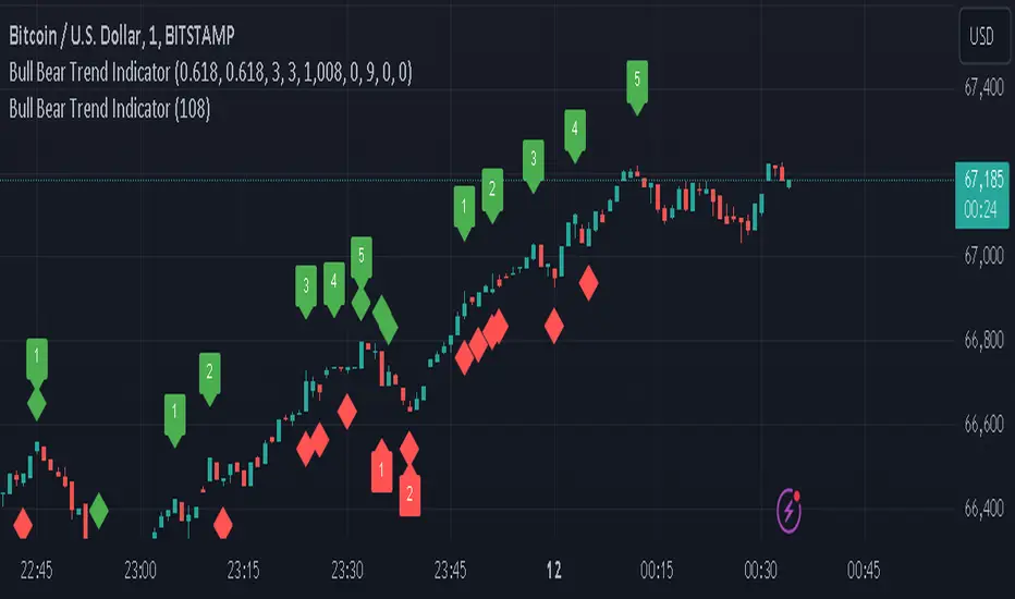
Bull Bear Trend IndicatorIntroduction: Origin of the Swing Point Indicator
In the quest for a reliable indicator that accurately predicts trend directions and identifies valid highs and lows, the genesis of the Swing Point Indicator emerged. Faced with the challenge of finding a tool that provided comprehensive market analysis and actionable insights, the need for a novel solution became evident. Combining insights gleaned from market analysis and innovative algorithmic approaches, the Swing Point Indicator was born.
Enhanced Feature: Highs and Lows Labeling in Trend Direction
In addition to its core functionalities, the Swing Point Indicator incorporates an advanced feature that enhances the visualization of trend direction. This feature provides further clarity by selectively labeling highs and lows based on the prevailing trend, reinforcing the identification of higher highs and lower lows in uptrends and downtrends, respectively. Overlapping labels on highs and lows signify a potential trend change, providing traders with valuable insight into market reversals.
Detailed Description:
1. Uptrend Labeling:
- Higher Highs (Green Label with Price): In an uptrend, where higher highs are observed, the indicator labels these points with vibrant green color and includes the corresponding price value. This visually highlights the significance of higher highs as pivotal points in the upward trajectory of prices.
- Higher Lows (Red Marker without Text or Diamond): To complement the identification of higher highs, higher lows are marked with a distinct red marker or diamond, devoid of any accompanying text. While these points are crucial in delineating the ascending trend, their emphasis lies in their role as support levels, providing a foundation for upward price movements.
2. Downtrend Labeling:
- Lower Lows (Red Label with Price): Conversely, in a downtrend characterized by lower lows, the indicator labels these points with conspicuous red color, accompanied by the corresponding price value. Lower lows signify critical levels of downward price momentum, acting as indicators of potential bearish continuation.
- Lower Highs (Green Marker without Text or Diamond): Lower highs, indicative of downward retracements in a downtrend, are marked by distinctive green markers or diamonds without accompanying text. While these points denote temporary pauses or pullbacks in the bearish trend, their emphasis lies in their role as resistance levels, impeding upward price movements.
Functionality and Utility:
- Customizable Lookback Candle Count: Traders have the option to adjust the lookback candle count, which is set by default at 108 candles in the settings. This flexibility allows traders to tailor the indicator to their specific trading preferences and timeframes.
- Equal Highs or Lows Option: When enabled, the Swing Point Indicator can identify equal highs or equal lows, providing traders with additional insight into market dynamics.
- Formation Confirmation: A new higher high along with its higher low or a new lower low along with its lower high is confirmed after two candles have closed following the swing point candle. This ensures the reliability of the identified trend direction.
Conclusion:
The incorporation of selective labeling for highs and lows based on trend direction, alongside the introduction of customizable settings and formation confirmation criteria, enhances the effectiveness of the Swing Point Indicator. This feature-rich tool empowers traders with a nuanced understanding of market dynamics, highlighting critical price levels and trend reversals. By offering enhanced visualization, customizable options, and confirmation criteria, the Swing Point Indicator equips traders with the confidence and precision needed to navigate the markets successfully, contributing to more informed and profitable trading strategies.
Multi-Timeframe Recursive Zigzag [Trendoscope®]🎲 Welcome to the Advanced World of Zigzag Analysis
Embark on a journey through the most comprehensive and feature-rich Zigzag implementation you’ll ever encounter. Our Multi-Timeframe Recursive Zigzag Indicator is not just another tool; it's a groundbreaking advancement in technical analysis.
🎯 Key Features
Multi Time-Frame Support - One of the rare open-source Zigzag indicators with robust multi-timeframe capabilities, this feature sets our tool apart, enabling a broader and more dynamic market analysis.
Innovative Recursive Zigzag Algorithm - At its core is our unique Recursive Zigzag Algorithm, a pioneering development that powers multiple Zigzag levels, offering an intricate view of market movements. This proprietary algorithm is the backbone of our advanced pattern recognition indicators.
Sub-Waves and Micro-Waves Analysis - Dive deeper into market trends with our Sub-Waves and Micro-Waves feature. Sub-Waves reveal the interconnectedness of various Zigzag levels, while Micro-Waves offer insight into the fundamental waves at the base level.
Enhanced Indicator Tracking - Integrate and track your custom indicators or oscillators with the zigzag, capturing their values at each Zigzag level, complete with retracement ratios. This offers a comprehensive view of market dynamics.
Curved Zigzag Visualization - Experience a new way of visualizing market movements with our Curved Zigzag Display, employing Pine Script’s polyline feature for a more intuitive and visually appealing representation.
Built-in Customizable Alerts - Stay ahead with built-in alerts that can be customized via user input settings.
🎯 Practical Applications
Our Zigzag Indicator is designed with an understanding of its inherent nature - the last unconfirmed pivot that consistently repaints. This characteristic, while by design, directs its usage more towards pattern recognition rather than direct identification of market tops and bottoms. Here's how you can leverage the Zigzag Indicator:
Harmonic Patterns - Ideal for those familiar with harmonic patterns, this tool simplifies the manual spotting of complex XABCD, ABC, and ABCD patterns on charts.
Chart Patterns - Effortlessly identify patterns like Double/Triple Taps, Head and Shoulders, Inverse Head and Shoulders, and Cup and Handle patterns with enhanced clarity. Navigate through challenging patterns such as Triangles, Wedges, Flags, and Price Channels, where the Zigzag Indicator adds a layer of precision to your breakout strategy.
Elliott Wave Components - The indicator's detailed pivot highlighting aids in identifying key Elliott Wave components, enhancing your wave analysis and decision-making process.
🎲 Deep Dive into Indicator Features
Join us as we explore the intricate features of our indicator in more detail.
🎯 Multi-Timeframe Capability
Our indicator comes equipped with an input option for selecting the desired resolution. This unique feature allows users to view higher timeframe Zigzag patterns directly on their lower timeframe charts.
🎯 Recursive Multi Level Zigzag
Our advanced recursive approach creates multi-level Zigzags from lower-level data. For instance, the level 0 Zigzag forms the base, calculated from specified length and depth parameters, while level 1 Zigzag is derived using level 0 as its foundation, and so forth.
The indicator not only displays multiple Zigzag levels but also offers settings to emphasize specific levels for more detailed analysis.
🎯 Sub-Components and Micro-Components of Zigzag Wave
Sub-components within a Zigzag wave consist of the previous level's Zigzag pivots. Meanwhile, the micro-components are composed of the base level (Level 0) Zigzag pivots encapsulated within the wave.
🎯 Curved Zigzag
Experience a new perspective with our curved Zigzag display. This innovative feature utilizes the polyline curved option to automatically generate sinusoidal waves based on multiple points.
🎯 Indicator Tracking
Default indicators such as RSI, MFI, and OBV are included, alongside the ability to track one external indicator at each Zigzag pivot.
🎯 Customizable Alerts
Our indicator employs the `alert()` function for alert creation. While this means the absence of a customization text box in the alert settings, we've included a custom text area for users to create their own alert templates.
Template placeholders include:
{alertType} - type of alert. Either Confirmed Pivot Update or Last Pivot Update. Depends on the alert type selected in the inputs.
When Last Pivot Update type is selected, the alerts are triggered whenever there is a new Zigzag Pivot. This may also be a repaint of last unconfirmed pivot.
When Confirmed Pivot Update type is selected, the alerts are triggered only when a pivot becomes a confirmed pivot.
{level} - Zigzag level on which the alert is triggered.
{pivot} - Details of the last pivot or confirmed pivot including price, ratio, indicator values and ratios, subcomponent and micro-component pivots.
🎲 User Settings Overview
🎯 Zigzag and Generic Settings
This involves some generic zigzag calculation settings such as length, depth, and timeframe. And few display options such as theme, Highlight Level and Curved Zigzag. By default, zigzag calculation is done based on the latest real time bar. An option is provided to disable this and use only confirmed bars for the calculation.
Indicator Settings
Allows users to track one or more oscillators or volume indicators. Option to add any indicator via external input is provided.
🎯 Alert Settings
Has input fields required to select and customize alerts.

Volatility Percentile (H-LINES)A simple script that adjusts the Volatility Percentile Indicator visibly in order to better accommodate entries/exits and certain trading setups/strategies.
--------------------------------------------------------------------------------------------------------------------------------------------------------
TL;DR - Remember after a full reset, we are looking for initial crosses UP on the UpperSwingline and crosses DOWN on the LowerSwingline for primary and secondary signal derivation.
Vice versa also works great but the prior method mentioned is a little more consistent in my experience, but you should mess around and optimise this for your own setups and strategies anyway.
--------------------------------------------------------------------------------------------------------------------------------------------------------
ORIGINAL SCRIPT HERE:
^Click image for a redirect to that script.
ALL CREDIT GOES TO: www.tradingview.com
He wrote everything so give credit where it's due, good bit of kit this here script is.
--------------------------------------------------------------------------------------------------------------------------------------------------------
HOW I USE MY VISUALLY ALTERED VERSION OF THIS SCRIPT
First of all, the alterations I've made seem only to be consistently viable with renko charts though if you can get the sought after results using candles or any other chart type then perfect, but be wary. All my back-testing done only with LinReg, HMA and SWMA - ATR type settings exclusively on renko charts. The changes I've made to the original script essentially just turns it visibly into an oscillator and uses a couple horizontal lines to generate signals, very simple - absolutely nothing has changed in the actual code of calculating this indicator.
What I believe my adjustments have achieved is quite simple. A full reset/oscillation on the indicator tries to map the strongest parts of a move or at least the part of the move where volume and the rate of transactions is at its peak to even facilitate said move. *take this statement with a pinch of salt though I do believe it's interacting with accumulation/distribution patterns, which is expected of volatility*
For ease of communication let's refer to the area between the the first UpperSwingline cross to the subsequent LowerSwingline cross, as the primary move. Then afterwards when it crosses the UpperSwingline again to make the full reset, the area in between those two points referred to as the secondary move.
Though more interestingly/practically the indicator ends up giving you two signals. In order for this to work we have to first decide that a spike up in volatility which crosses the UpperSwingline implies a significant level of interest at that price level. Usually that means a reversal is brewing, if price has already moved, trended and is approaching a certain area of value; which causes a spike of new positions to be taken, then you know that this is a level where contrarians are looking to enter. Now here's the tricky part, when volatility crosses the LowerSwingline price action becomes a little more open for interpretation, the way I personally like to look at this secondary signal is the potential for an exhaustion period to prolong itself a little longer. I know that's not the perfect analysis for what's going on, a more in-depth look into what's going on would best be described using Elliott Wave Theory, if a cross on the UpperSwingline near a significant area of value gives us a reversal trade lets just assume for the sake of argument that a new Elliott Wave can begin forming here. Making the move from that initial UpperSwngline cross to the cross on the LowerSwingline, the area that encompasses those two points: the impulse wave. After this point my analogy kind of falls apart and sadly my knowledge just isn't what it needs to be in order for me to properly analyse what's going on here but I must digress. Price after crossing the LowerSwingline up until the point where it makes a full reset by crossing the UpperSwingline again, within this area price seems to do either one of two things:
Situation 1 - Most likely occurs after a major trend reversal from major support/resistance or area of value (price has trended to new territory, maybe spent time a little time consolidating but hasn't broken the key level, momentum shifts, price action breaks current structure and you get the signal that primary move is a reversal) = Exhaustion Period, price will continue in direction of primary move during the secondary move. This here is for our trend-followers, you wanna take a continuation trade? Just wait for the pullback/rally to hit a FiB retracement level and enter - or any other means to find a decent support/resistance to enter.
Situation 2 - Most likely occurs when market enters a range or consolidation (price was previously seen as being at either a discount or premium so Situation 1 could have already played out and now you're looking at a full reset after that, imagine this spot to be the centre line of a linear regression channel or bang in the middle of your range, could even occur if price breaks a key moving average and decides it ought to consolidate around it for a while. Basically at any point where a somewhat prolonged consolidation is expected and not a quick reversal) = Corrective Wave, price will move against the direction of primary move during the secondary move. Now you might be expecting me to say this ones for you reversal traders but not really, if this is occurring then there probably isn't a definitive direction the market has chosen so you can use this opportunity to take range trades in the direction or against the direction of whatever the current trend or latest trend was depending on whatever slight bias you may have. <--- Situation 2 is very useful for finding cleaner entries if you do have a trend bias, say price underwent Situation 1, is now at key moving average but your bias is that it will break and continue up, so you wait and allow the secondary move of Situation 2 to take your entry to a much better R:R before entering a position.
--------------------------------------------------------------------------------------------------------------------------------------------------------

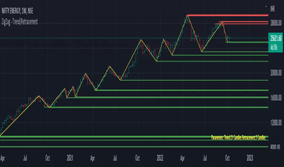
Trend/Retracement - ZigZag - New wayZigZag for Trend and Retracements - New way
It's another way to plot ZigZag based on lookback period for trend and % of trend lookback period to plot retracements.
█ OVERVIEW
Plot ZigZag, Trend lines, Retracements, Support levels, Resistance levels
█ Objective:
Draw ZigZag lines along with unbroken support and resistance levels. ZigZag lines are drawn for main trend and the retracements.
Main Trend – This is calculated based on lookback period.
Retracements – Retracements are calculated as 25% of main trend.
Support and Resistance line: The indicator draws 2 types of support and resistance lines
1. Un-broken – Once formed (plotted), these are the support and resistance which are not yet broken
2. Tested – One can also choose to see support and resistance lines which are tested but not broken. Tested support/resistance are those levels which are touched by high/low price but close price has not crossed the level.
█ How main trend point is calculated:
E.g.
Chart timeframe = 15m
Lookback period = 250
Retracement = 25% of main trend ( 25% of 250 = 62 )
A price point on a chart is considered as trend point if distance between current price and previous highest price is 250 candles
A price point is considered as a retracement if distance between current price and previous highest price is 62 candles. Please note retracements are calculated only after finding a main trend point.
█ Input parameters:
Zigzag Parameters
Use predefined Lookback – If checked pre-defined timeframe-based lookback parameters are used.
Trend lookback candles – If ‘Use predefined Lookback’ is unchecked then this value is used as lookback period.
Retracement % of look back candles– If ‘Use predefined Lookback’ is unchecked then this value is used for calculating retracement lookback period
Mark retracements – If unchecked only main trend lines are plotted
Plot support/resistance – To plot support/resistance levels
Show support/resistance tested lines – If checked tested support/resistance liens are shown on the chart
█ TF based Lookback period config (Defaults are set as specified below, One can change these defaults to use different lookback periods)
The defaults set here are used based on the chart timeframe. e.g. if chart timeframe is changed from say 15m to 60m then 60m chart defaults (i.e. trend lookback = 90) are used to plot the trend and the retracements. At the bottom-right of the chart, parameters used for plotting are displayed all the time.
Timeframe in minute – Default = 5m
Trend lookback candles – Default = 375 (~ 5 days of data)
Timeframe in minute – Default = 15m
Trend lookback candles – Default = 250 (~10 days of data)
Timeframe in minute – Default = 60m
Trend lookback candles = Default = 90 (~ 15 days of data)
Trend lookback candles for timeframe 'D' – Default = 30 (~1 month data)
Trend lookback candles for timeframe 'W' – Default = 21 (~6 months data)
Trend lookback candles for timeframe 'M' – Default = 12 (~1year data)
Retracement % of look back candles – Default = 25%
█ When and where one can use this indicator (Refer to chart examples)
To view support and resistance based on lookback period
To view ZigZag lines
One can use it to find chart patterns easily
Trend and retracement lines can help in drawing Elliott waves.
█ Chart examples:
1. Chart patterns can be easily identified - One can disable the candle charts which will help to identify and draw chart patterns easily
2. Trend and retracement lines can also help is analyzing charts (e.g. Elliott Waves can be marked based on trend lines)
3. Tested but not broken support and resistance lines can be viewed
4. You can select 'NOT' to plot tested support and resistance lines
5. Uncheck the Mark retracements to plot main trend lines (Retracements are not marked)
CDC Fibonacci Retracement and ExtensionThis indicator is meant to be used as a tool to quickly identify
fibonacci retracements and projections in multiple charts during
the same date range.
Users can set the calculation date range and quickly flip through
different charts for comparisons
Steps for using this indicator is as follows:
1. Specify Start Date and End Date for calculations
2. Choose Open-ended mode for just retracements, this will disregard
end date in calculations.
3. Select price source, if Use Highs/Lows is selected, the indicator will
use high and low prices for calculation, if not, closing price eill
be used instead
4. Select and/or modify retracement / projection lines as you see fit.
5. Enjoy the result!

Bitcoin Golden Bottom Oscillator (MZ BTC Oscillator)This indicator uses Elliot Wave Oscillator Methodology applied on "BTC Golden Bottom with Adaptive Moving Average" and Relative Strength Index of Resulted EVO to form an Oscillator to detect trend health in Bitcoin price. Ticker is set to "INDEX : BTCUSD" on 1D timeframe.
Methodology
Oscillator uses Adaptive Moving Average with 1 year of length, Minor length of 50 and Major length of 100 to mark AMA as Golden Bottom.
Percentage Elliot Wave Oscillator is calculated between BTC price and AMA.
Relative Strength Index of EVO is calculated to detect trend strength and divergence detection.
Hull Moving Average of resulted RSI is used to smoothen the Oscillator.
Oscillator is hard coded to 'INDEX:BTCUSD' ticker on 1d so it can be used on any other chart and on any other timeframe.
Color Schemes
Bright Red background color indicates that price has left top Fib multiple ATR band and possibly go for top.
Light Red background color indicates that price has left 2nd top Fib multiple ATR band and possibly go for local top.
Lime background color indicates that price has entered lowest band indicating local bottom.
Bright Green background color indicates that price is approximately resting on Golden Bottom i.e. AMA.
Oscillator color is set to gradient for easy directional adaption.
BTC Golden Bottom with Adaptive Moving Average

Cavuca Technical AnalysisScript created by Cavuca-Trader for technical analysis of various assets. It is based on analysis of moving averages and also on Elliot wave movements, signaling entries and exits through its own coloration.
Mode of Viewing the indicator: Moving averages are used to assist in the movement of the asset's trend by observing its slope. The indicator recognizes market movements and detects the tops and bottoms of the movement by creating horizontal lines. When candles break these lines they gain color according to the trend of the movement.
Notes in the author's language:
Script criado por Cavuca-Trader para análise técnica de diversos ativos . Basea-se em análise de médias móveis e também em movimentos das Ondas de Elliot , sinalizando entradas e saídas através de coloração própria.
Modo de Visualizar o indicador: As médias móveis servem para auxiliar na movimentação de tendência do ativo observando a sua inclinação. O indicador reconhece os movimentos do mercado e detecta os topos e fundos do movimento criando linhas horizontais. Quando os candles rompem essas linhas ganham a coloração de acordo com a tendência do movimento.

Multpile strategies [LUPOWN]///English
This indicator contains many indicators that together can form different strategies, by default there is the Latin trading strategy with the points of the cipher by @Vumanchu indicator that actually these points appear when a lazy bear indicator gives the signal, the white shadow that It is seen by default is the MFI, this adaptation is the same as the one with the indicator cipher by @Vumanchu, if the white shadow is above the 0 point we can search for a buy position, this helping us with the squeeze momentum and the ADX (information in the panel), you can even enter before the buy or sell panel if the green dot appears, this is one of several strategies that can be formed with this indicator.
Other hidden indicators by default are the CCi, Koncorde (adapted thanks to the version of @inversiones por el mundo and modified by @ lkdml), MACD, stochastic, Awesome Oscillator, Elliot Oscillator, which, as I say, combined can be good strategies.
The indicator also shows divergences, both in the RSI and in the Squeeze momentum and in the Awesome Oscillator if it is on the chart, the divergence code is from @madoqa and I adapted it for the different indicators.
The panel shows the status of the chart according to the Trading Latino strategy
You can hide and show the indicators you want through the settings.
///// Spanish
Este indicador contiene muchos indicadores que en conjunto pueden formar diversas estrategias, por default esta la estrategia de trading latino con los puntos del indicador cipher by @Vumanchu que en realidad estos puntos aparecen cuando un indicador de lazy bear da la señal, la sombra blanca que se ve por default es el MFI esta adaptación es la misma a la que tiene el indicador cipher by @Vumanchu, si la sombra blanca esta por encima del punto 0 podemos buscar entradas en compra, esto ayudándonos del squeeze momentum y el ADX (información en el panel), incluso se puede entrar antes que el panel nos de compra o venta si el punto verde aparece, esta es una de varias estrategias que se pueden formar con este indicador.
Otros indicadores ocultos por default están el CCi, Koncorde (adaptado gracias a la versión de @inversiones por el mundo y modificado por @ lkdml), MACD, estocastico , Awesome Oscillator, Elliot Oscilator, que como digo combinados se pueden hacer buenas estrategias.
En el indicador también se muestran divergencias, tanto en el RSI como en el Squeeze momentum y en el Awesome Oscillator si es que esta en el grafico, el código de divergencias es de @madoqa yo lo adapte para los diferentes indicadores.
El panel muestra el estatus del grafico según la estrategia de Trading Latino
Puedes ocultar y mostrar los indicadores que quieras mediante las configuraciones.

Time Wolna_2021_iun3[wozdux] Description of the Time_Wolna indicator
The indicator is designed to study the behavior of time. There are many indicators that study just the price, a little less indicators that study the volume of trading and vanishingly few indicators that study time.
This is not an oscillator, it does not have oversold or overbought levels. This indicator has an indefinite beginning and an indefinite end. Its value is not in the absolute values of the indicator, but in relative ones. This indicator calculates the time of price rise and the time of price decline. It clearly shows how long the price rises and how long the price falls.
The initial idea was to use my RSIVol indicator to study the time. Each bar is counted as a unit of time. If the price rises during the period of one bar, then one is added, if the price falls, then one is subtracted. By default, the blue line shows this time movement according to the RsiVol indicator.
The basic RsiVol indicator is shown at the bottom of the diagram. The bill goes along the blue line, which calculates the movement of the volume price. If the blue RSIVol line is above the yellow level, then the blue Time_Wolna time line is colored green. If the blue line in the base RsiVol indicator falls below the lower yellow level, then the blue time line of the Time_Wolna indicator turns red.
The result is a broken line that clearly shows the waves of rising and falling prices. In principle, the time indicator makes it easier to recognize waves.
It is known that time plays an important role in Elliott wave analysis, although in practice this is almost never done. The mention of Elliott is just a lyrical digression.
Time is very difficult to study. This indicator does not give clear buy or sell signals. This is just an analysis tool to help analysts.
In addition to the RsiVol indicator, simply the Rsi from the price and a simple moving average from the price are also used.
So, the settings of this indicator.
"switch Price == close <==> ( High+Low)/2" -- select the base price in all subsequent calculations
"Key EMA=> True=ema(Price); False=ema(Price*Volume)" --The key for switching the moving average from the price or from the volume price.
"T==> EMA(price, T)" --The period for calculating the moving average
" key red==> Yes/No Rsi")--the key turns on or off the RSI line red line
"key green==> Yes/No Orsi") --the key turns on or off the Volume RSI line green line
" key olive==> Yes/No RsiVol200 " -- the key enables or disables the Volumetric RSIVol200 olive line. This is RsiVol minus the 200-period moving average.
"keyVol blue==> Yes/No " - the key enables or disables the base blue line RSIVol
"keyVol blue==> V->tt(RsiVol) ->tt(ema(Price))"—The blue line selection will be calculated as the time from RSIVol or as the time from the moving average EMA.
"keyVol blue==> : 1=Time, 2=Time* price, 3=Time*(Ci-Ck) 4=Time*Volume, 5=Time*price*Volume")- selection for the blue baseline. By default, the time of the price rise or fall is calculated simply. Key=1. But you can investigate the joint influence of time and price and then the key is=2. If we study the combined effect of time and price changes per bar, then the key=3. If we study the joint influence of time and volume, then the key=4. If we study the joint influence of time, price and volume, then the key=5.
"key RsiO red + green==> : 1=Time, 2=Time*Price, 3=Time*(Ci-Ck) 4=Time*Volume, 5=Time*Price*Volume") - - - similar settings for the red green line. By default, the time of the price rise or fall is calculated simply. Key=1. But you can investigate the joint influence of time and price and then the key is=2. If we study the combined effect of time and price changes per bar, then the key=3. If we study the joint influence of time and volume, then the key=4. If we study the joint influence of time, price and volume, then the key=5.
"Key Color – - here you can disable changing the color of the blue line to green or red when the base indicator RsiVol exits above the upper and below the lower levels.
"Level nul ==> * Down Level Rsi - screen configuration in order to raise or lower chart
"Level nul ==> * Down Level ORsi -- beauty setup in order to raise or lower chart
"Level nul ==> * DownLevel RsiVol200 -- beauty setup in order to raise or lower chart
"blue =volume * price" – period for calculation of volumetric rates
"blue => RSIVOL(Volume*price,len) and EMA" – the period for calculating RsiVol
"blue__o1=> ema ( RSIVOL, o1)" – additional smoothing RsiVol
"red=rsi (Price,14)" – the period for calculating Rsi
"red= ema ( RSI ,3)" -- additional smoothing Rsi
"fuchsia__ => RsiVol200 (vp,200)" - the period for calculating RsiVol200
"fuchsia__o2=> ema ( RSIVOL200 , o2)" -- additional smoothing RsiVol200
To study the time between two fixed dates. Setting the start point of the calculation and the end point of the calculation
"Data(0)=Year" – the year of the start date
"Data(0)= Month" – the month of the start date
"Data (0)=Day" the day of the start date
"Data(1)=Year" – the year of the end date.
"Data(1)=Year" – month of the end date.
"Data(1)=Day" -- the day of the end date.
--------русский вариант описания ------
Описание индикатора Time_Wolna
Индикатор призван изучать поведение времени. Есть много индикаторов изучающих просто цену, немного меньше индикаторов изучающих объем торгов и исчезающе мало индикаторов, изучающих время.
Это не осциллятор у него нет уровней перепроданности или перекупленности. Данный индикатор имеет неопределенное начало и неопределенный конец. Ценность его не в абсолютных значениях индикатора, а в относительных. Этот индикатор высчитывает время подъема цены и время снижения цены. Он наглядно показывает сколько времени цена поднимается и сколько времени цена опускается.
Первоначальная идея была использовать мой индикатор RSIVol для изучения времени. Каждый бар считается за единицу времени. Если цена поднимается за период одного бара, то прибавляется единица, если цена опускается, то вычитается единица. По умолчанию голубая линия показывает такое движения времени по индикатору RsiVol.
Внизу на диаграмме показан базовый индикатор RsiVol. Счёт идет по синей линии, которая вычисляет движение объемной цены. Если синяя линия RSIVol находится выше желтого уровня, то голубая линия времени Time_Wolna окрашивается в зеленый цвет. Если синяя линия в базовом индикаторе RsiVol опускается ниже нижнего желтого уровня, то голубая линия времени индикатора Time_Wolna окрашивается в красный цвет.
В результате получается ломанная линия, четко показывающая волны восхождения и снижения цены. В принципе индикатор времени позволяет легче распознавать волны.
Известно, что время играет важную роль в волновом анализе Эллиотта, хотя на практике это почти никогда не делается. Упоминание Эллиотта это просто лирическое отступление.
Время очень трудно изучать. Этот индикатор не дает четких сигналов на покупку или продажу. Это всего лишь инструмент анализа в помощь аналитикам.
Кроме индикатора RsiVol, используются и просто Rsi от цены и простая скользящая средняя от цены.
Итак, настройки данного индикатора.
"switch Price == close <==> ( High+Low)/2" -- выбираем базовую цену во всех последующих вычислениях
"Key EMA=> True=ema(Price); False=ema(Price*Volume)" --Ключ переключения скользящей средней от цены или от объемной цены.
" T==> EMA(price,T)"--Период вычисления скользящей средней
"key red==> Yes/No Rsi")--ключ включает или выключает линию RSI красная линия
"key green==> Yes/No Orsi") --ключ включает или выключает линию Объемной RSI зеленая линия
"key olive==> Yes/No RsiVol200" -- ключ включает или выключает линию Объемной RSIVol200 оливковая линия. Это RsiVol минус 200-периодная скользящая средняя.
"keyVol blue==> Yes/No " – ключ включает или выключает базовую голубую линию RSIVol
"keyVol blue==> V->tt(RsiVol) ->tt(ema(Price))"—выбор голубая линия будет вычисляться как время от RSIVol или как время от скользящей средней EMA.
"keyVol blue==> : 1=Time, 2=Time* price, 3=Time*(Ci-Ck) 4=Time*Volume, 5=Time*price*Volume")—выбор для голубой базовой линии. По умолчанию вычисляется просто время подъема или опускания цены. Ключ=1. Но можно исследовать совместное влияние времени и цены и тогда ключ=2. Если изучаем совместное влияние времени и изменения цены за один бар, то ключ=3. Если изучаем совместное влияние времени и объема, то ключ=4. Если изучаем совместное влияние времени, цены и объема, то ключ=5.
"key RsiO red + green==> : 1=Time, 2=Time*Price, 3=Time*(Ci-Ck) 4=Time*Volume, 5=Time*Price*Volume") ---аналогичные настройки для красной зеленой линии. По умолчанию вычисляется просто время подъема или опускания цены. Ключ=1. Но можно исследовать совместное влияние времени и цены и тогда ключ=2. Если изучаем совместное влияние времени и изменения цены за один бар, то ключ=3. Если изучаем совместное влияние времени и объема, то ключ=4. Если изучаем совместное влияние времени, цены и объема, то ключ=5.
"Key Color" – здесь можно отключить изменение цвета голубой линии на зеленый или красный в моменты выхода базового индикатора RsiVol выше верхнего и ниже нижнего уровней.
"Level nul ==> * Down Level Rsi - косметическая настройка для того, чтобы поднять или опустить график
"Level nul ==> * Down Level ORsi -- косметическая настройка для того, чтобы поднять или опустить график
"Level nul ==> * DownLevel RsiVol200 -- косметическая настройка для того, чтобы поднять или опустить график
" blue =>volume * price" – период для вычисления объемной цены
" blue => RSIVOL(Volume*price,len) and EMA" – период для вычисления RsiVol
"blue__o1=> ema ( RSIVOL, o1)" – дополнительное сглаживание RsiVol
" red=rsi (Price,14)" – период для вычисления Rsi
" red= ema ( RSI ,3)" -- дополнительное сглаживание Rsi
"fuchsia__ => RsiVol200 (vp,200)" -- период для вычисления RsiVol200
"fuchsia__o2=> ema ( RSIVOL200 , o2)" -- дополнительное сглаживание RsiVol200
Для исследования времени между двумя фиксированными датами. Задаем начальную точку вычисления и конечную точку вычисления
"Data(0)=Year" – год начальной даты
"Data(0)= Month" – месяц начальной даты
"Data(0)=Day" день начальной даты
"Data(1)=Year" – год конечной даты.
"Data(1)=Year" – месяц конечной даты.
"Data(1)=Day" -- день конечной даты.

High/low crypto strategy with MACD/PSAR/ATR/EWaveToday I am glad to bring you another great creation of mine, this time suited for crypto markets.
MARKET
Its a high and low strategy, designed for crypto markets( btcusd , btcusdt and so on), and suited for for higher time charts : like 1hour, 4hours, 1 day and so on.
Preferably to use 1h time charts.
COMPONENTS
Higher high and lower low between different candle points
MACD with simple moving average
PSAR for uptrend and downtrend
Trenddirection made of a modified moving average and ATR
And lastly elliot wave oscillator to have an even better precision for entries and exits.
ENTRY DESCRIPTION
For entries we have : when the first condition is meet(we have a succession on higher high or lower lows), then we check the macd histogram level, then we pair that with psar for the direction of the trend, then we check the trend direction based on atr levels with MA applied on it and lastly to confirm the direction we check the level of elliot wave oscillator. If they are all on the same page we have a short or a long entry.
STATS
Its a low win percentage , we usually have between 10-20% win rate, but at the same time we use a 1:30 risk reward ratio .
By this we achieve an avg profit factor between 1.5- 2.5 between different currencies.
RISK MANAGEMENT
In this example, the stop loss is 0.5% of the price fluctuation ( 10.000 -> 9950 our sl), and tp is 15% (10.000 - > 11500).
In this example also we use a 100.000 capital account, risking 5% on each trade, but since its underleveraged, we only use 5000 of that ammount on every trade. With leveraged it can be achieved better profits and of course at the same time we will encounter bigger losses.
The comission applied is 5$ and a slippage of 5 points aswell added.
For any questions or suggestions regarding the script , please let me know.
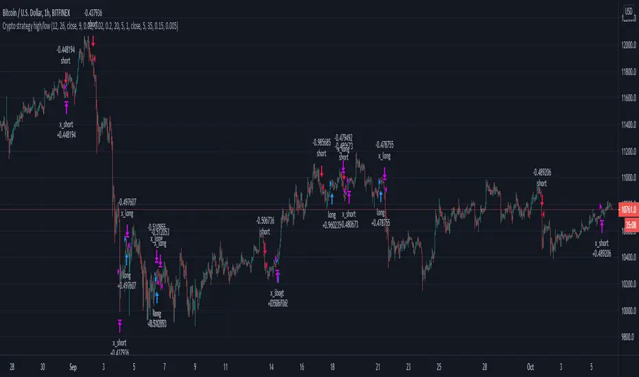
SMA/pivot/Bollinger/MACD/RSI en pantalla gráficoMulti-indicador con los indicadores que empleo más pero sin añadir ventanas abajo.
Contiene:
Cruce de 3 medias móviles
La idea es no tenerlas en pantalla, pero están dibujadas también. Yo las dejo ocultas salvo que las quiera mirar para algo.
Lo que presento en pantalla es la media lenta con verde si el cruce de las 3 marca alcista, amarillo si no está claro y rojo si marca bajista.
Pivot
Normalmente los tengo ocultos pero los muestro cuando me interesa. Están todos aunque aparezcan 2 seguidos.
Bandas de Bollinger
No dibujo la línea central porque empleo la media como tal.
Parabollic SAR
Lo empleo para dibujar las ondas de Elliott como postula Matías Menéndez Larre en el capítulo 11 de su libro "Las ondas de Elliott". Así que, aunque se puede mostrar, lo mantengo oculto y lo que muestro es dónde cambia (SAR cambio).
MACD
No está dibujado porque necesitaría sacarlo del gráfico.
Marco en la parte superior cuándo la señal sobrepasa al MACD hacia arriba o hacia abajo con un flecha indicando el sentido de esta señal.
RSI
Similar al MACD pero en la parte inferior.
Probablemente, programe otro indicador para visualizar en una ventanita MACD, RSI y volumen todo junto. El volumen en la principal hay veces que no te permite ver bien alguna sombra y los otros 2 te quitan mucho espacio para graficar si los tienes permanentemente en 2 ventanas separadas.
Bill Williams Trading Chaos Vol 1-NoviceThis is a revision of a script developed by tekolo. I hope tekolo takes a look. The concepts are here but I struggle with pine. I am very much a novice, but I tried to put information from the original book, Trading Chaos, Volume One by Bill Williams. There are too many plots to get this to wor. I made a lot of plot lines into comments to get it to run. I'm hoping someone with an interest in this material and some programming skills will be kind enough to take these thoughts and put them in a script that the Pine Editor would actually run. Thanks for taking a look. I do believe in these leading indicators. This is information included for Novice Level Trading in the Bill Williams book. There are more indicators developed in his material, but the jest is that Price is an end result of the marketplace. Market participation (Volume), Market Bias (Momentum), Increased Participation and Bias (Acceleration) all preceed the formation of the Trend. This along with Elliott Wave interpretation using his indicators as a basis for locating key points of the Elliott Wave, are most of what I understand about this interesting man's work. Again, I am a novice at all of this, but the leading indicators that result in price seem interesting. Thanks!
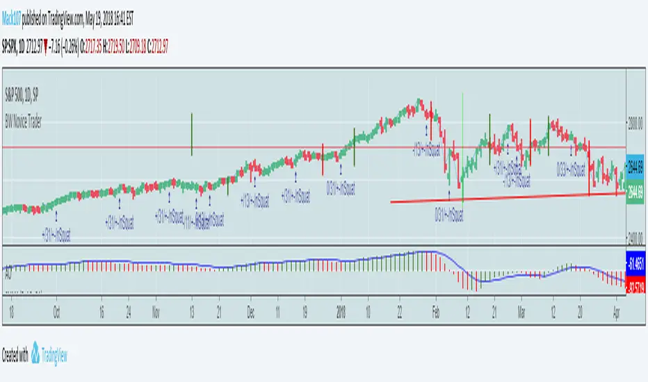
VaRz BTC/Gold Risk MeterVaRz Risk Meter (BTC vs Risk-On & Gold Safe-Haven Proxy)
The VaRz Risk Meter is a macro sentiment oscillator designed to measure Bitcoin’s relative strength and directional bias using key risk-appetite and safe-haven flows.
Indicator Components
VIX → Market fear & volatility benchmark
NASDAQ 100 (NDX) → Primary risk-on proxy (growth/tech capital flow)
Gold (XAUUSD) → Safe-haven strength alternative to USD index
Bitcoin (BTCUSDT) → Used only for normalization reference, not bias calculation
Core Logic
All assets are normalized on a 0–100 scale using a 100-period rolling window to create a balanced comparison across markets.
The Bitcoin Macro Bias Histogram is calculated as:
NASDAQ strength − VIX fear − Gold safe-haven strength
This produces a macro directional regime for Bitcoin:
Market Regimes Interpretation
Indicator State Meaning for BTC
NASDAQ high + VIX low + Gold weak Risk-On environment → Bullish for Bitcoin
Gold strong + VIX rising + NASDAQ weak Risk-Off / flight to safety → Bearish pressure on BTC
All assets near 50 with no trend Neutral / Sideways → Macro indecision
How to Use
This is not a direct entry signal, but a macro bias filter
Best combined with:
Market Structure, Liquidity zones, Orderflow, Volume analysis, and Elliott Wave context
Bias becomes more reliable on higher timeframes (1W, 1M) but works on any chart
Key Insight
Bitcoin behaves as a hybrid risk asset. This indicator helps track when capital is:
Rotating into risk markets (favorable for BTC)
or
Seeking protection in gold and volatility hedges (unfavorable for BTC)
The histogram visually maps these shifts to give traders a clear macro regime awareness in one window.

DANGHIEU EMA 34/89/200 Ribbon (Scaled HTF)📘 Indicator Description – EMA 34/89/200 Ribbon (Scaled HTF)
The EMA 34/89/200 Ribbon (Scaled HTF) indicator is designed to replicate higher-timeframe EMAs directly on your current chart without switching timeframes.
Using a precise HTF Scaling Algorithm, the script converts EMAs from 1H, 2H, 4H, 6H, 12H, 1D, and even 1W into equivalent lengths on lower timeframes—allowing traders to perform true multi-timeframe trend analysis on a single chart.
The 34-EMA and 89-EMA form a dynamic trend ribbon that changes color based on the relationship between the two moving averages. This helps traders quickly identify trend direction, momentum strength, and potential market reversals. The indicator also includes optional crossover markers (X symbols) to highlight bullish and bearish crossovers for cleaner signal recognition. EMA200 is included as the long-term trend anchor.
This tool is ideal for scalpers, day traders, and swing traders who require higher-timeframe context while trading lower-timeframe entries.
🟦 How to Use the Indicator
1. Choose the Higher Timeframe to Simulate
Use the “HTF to Simulate” dropdown to select the timeframe you want to emulate (e.g., 4H, 2H, 1D, 1W).
The script automatically scales the EMA lengths so they match the selected HTF.
2. Read the Ribbon for Trend Direction
Green Ribbon → EMA34 above EMA89 → Bullish momentum
Red Ribbon → EMA34 below EMA89 → Bearish momentum
The ribbon expands when momentum strengthens and contracts during consolidation.
3. Use EMA Crossovers as Signal Zones
Optional X markers highlight crossover points:
Bullish Crossover → EMA34 crosses above EMA89
Bearish Crossover → EMA34 crosses below EMA89
These crossovers often align with trend shifts or early momentum changes.
4. EMA200 as Trend Filter
The EMA200 acts as the macro trend filter:
Price above EMA200 → only consider long setups
Price below EMA200 → only consider short setups
Combining ribbon trend + EMA200 alignment improves signal accuracy.
5. Multi-Timeframe Trading Strategy
This indicator is powerful for:
Scalping with HTF bias
Pullback entry on lower timeframe during HTF trend
Identifying trend exhaustion when the ribbon flips
Confirming wave structure (Elliott Wave, Dow Theory)
Spotting strong momentum phases and squeeze zones
Example workflow:
Select 4H as HTF simulation.
Trade on 15m or 5m chart.
Enter only when price aligns with the HTF ribbon + EMA200 trend.
Use EMA crossovers as confirmation signals.

Risk-On / Risk-Off Composite (Elliot) – Macro+Vol Upgrade v2drop-in upgrade of indicator that adds three optional macro components with adjustable weights:
Inverted VIX (risk-on when down → we use 100/VIX)
Inverted MOVE (bond vol; risk-on when down → we use 1/MOVE)
Inverted DXY (USD; risk-on when down → we use 1/DXY)

Constance Brown Composite Index EnhancedWhat This Indicator Does
Implements Constance Brown's copyrighted Composite Index formula (1996) from her Master's thesis - a breakthrough oscillator that solves the critical problem where RSI fails to show divergences in long-horizon trends, providing early warning signals for major market reversals.
The Problem It Solves
Traditional RSI frequently fails to display divergence signals in Global Equity Indexes and long-term charts, leaving asset managers without warning of major price reversals. Brown's research showed RSI failed to provide divergence signals 42 times across major markets - failures that would have been "extremely costly for asset managers."
Key Components
Composite Line: RSI Momentum (9-period) + Smoothed RSI Average - the core breakthrough formula
Fast/Slow Moving Averages: Trend direction confirmation (13/33 periods default)
Bollinger Bands: Volatility envelope around the composite signal
Enhanced Divergence Detection: Significantly improved trend reversal timing vs standard RSI
Research-Proven Performance
Based on Brown's extensive study across 6 major markets (1919-2015):
42 divergence signals triggered where RSI showed none
33 signals passed with meaningful reversals (78% success rate)
Only 5 failures - exceptional performance in monthly/2-month timeframes
Tested on: German DAX, French CAC 40, Shanghai Composite, Dow Jones, US/Japanese Government Bonds
New Customization Features
Moving Average Types: Choose SMA or EMA for fast/slow lines
Optional Fills: Toggle composite and Bollinger band fills on/off
All Periods Adjustable: RSI length, momentum, smoothing periods
Visual Styling: Customize colors and line widths in Style tab
Default Settings (Original Formula)
RSI Length: 14
RSI Momentum: 9 periods
RSI MA Length: 3
SMA Length: 3
Fast SMA: 13, Slow SMA: 33
Bollinger STD: 2.0
Applications
Long-term investing: Monthly/2-month charts for major trend changes
Elliott Wave analysis: Maximum displacement at 3rd-of-3rd waves, divergence at 5th waves
Multi-timeframe: Pairs well with MACD, works across all timeframes
Global markets: Proven effective on equities, bonds, currencies, commodities
Perfect for serious traders and asset managers seeking the proven mathematical edge that traditional RSI cannot provide.
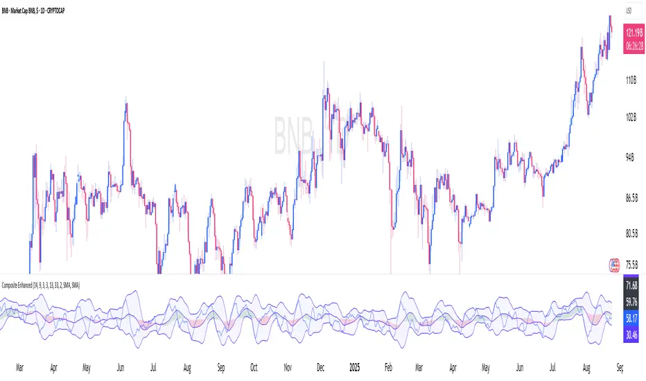
SCPEM - Socionomic Crypto Peak Model (0-85 Scale)SCPEM Indicator Overview
The SCPEM (Socionomic Crypto Peak Evaluation Model) indicator is a TradingView tool designed to approximate cycle peaks in cryptocurrency markets using socionomic theory, which links market behavior to collective social mood. It generates a score from 0-85 (where 85 signals extreme euphoria and high reversal risk) and plots it as a blue line on the chart for visual backtesting and real-time analysis.
#### How It Works
The indicator uses technical proxies to estimate social mood factors, as Pine Script cannot fetch external data like sentiment indices or social media directly. It calculates a weighted composite score on each bar:
- Proxies derive from price, volume, and volatility data.
- The raw sum of factor scores (max ~28) is normalized to 0-85.
- The score updates historically for backtesting, showing mood progression over time.
- Alerts trigger if the score exceeds 60, indicating high peak probability.
Users can adjust inputs (e.g., lengths for RSI or pivots) to fine-tune for different assets or timeframes.
Metrics Used (Technical Proxies)
Crypto-Specific Sentiment
Approximated by RSI (overbought levels indicate greed).
Social Media Euphoria
Based on volume relative to its SMA (spikes suggest herding/FOMO).
Broader Social Mood Proxies
Derived from ATR volatility (high values signal uncertain/mixed mood).
Search and Cultural Interest Proxied by OBV trend (rising accumulation implies growing interest).
Socionomic Wildcard
Uses Bollinger Band width (expansion for positive mood, contraction for negative).
Elliott Wave Position
Counts recent price pivots (more swings indicate later wave stages and exhaustion).