Bitcoin Fundamentals - Puell MultipleThis is an indicator that derives from Bitcoin Mining daily generated Income.
It does show a perfect track record on calling Bitcoin cycle tops and cycle bottoms.
For those of you willing to experiment, I've enabled the ability to set custom periods (365 by default).
The indicator includes custom alerts to notify the entry and the exit from OverBought (OB) & OverSold (OS) bands.
Credits: David Puell twitter.com
Wyszukaj w skryptach "Cycle"
Cycle Dynamic Composite AverageThis MA uses the formula of simple cycle indicator to find 2 cycles periods length's .
The CDCA is the result of 8 different ma to control and filter the price. The regression line is the signal , don t need to look candles, but just the cross between MA and reg lin.
TASC 2025.06 Cybernetic Oscillator█ OVERVIEW
This script implements the Cybernetic Oscillator introduced by John F. Ehlers in his article "The Cybernetic Oscillator For More Flexibility, Making A Better Oscillator" from the June 2025 edition of the TASC Traders' Tips . It cascades two-pole highpass and lowpass filters, then scales the result by its root mean square (RMS) to create a flexible normalized oscillator that responds to a customizable frequency range for different trading styles.
█ CONCEPTS
Oscillators are indicators widely used by technical traders. These indicators swing above and below a center value, emphasizing cyclic movements within a frequency range. In his article, Ehlers explains that all oscillators share a common characteristic: their calculations involve computing differences . The reliance on differences is what causes these indicators to oscillate about a central point.
The difference between two data points in a series acts as a highpass filter — it allows high frequencies (short wavelengths) to pass through while significantly attenuating low frequencies (long wavelengths). Ehlers demonstrates that a simple difference calculation attenuates lower-frequency cycles at a rate of 6 dB per octave. However, the difference also significantly amplifies cycles near the shortest observable wavelength, making the result appear noisier than the original series. To mitigate the effects of noise in a differenced series, oscillators typically smooth the series with a lowpass filter, such as a moving average.
Ehlers highlights an underlying issue with smoothing differenced data to create oscillators. He postulates that market data statistically follows a pink spectrum , where the amplitudes of cyclic components in the data are approximately directly proportional to the underlying periods. Specifically, he suggests that cyclic amplitude increases by 6 dB per octave of wavelength.
Because some conventional oscillators, such as RSI, use differencing calculations that attenuate cycles by only 6 dB per octave, and market cycles increase in amplitude by 6 dB per octave, such calculations do not have a tangible net effect on larger wavelengths in the analyzed data. The influence of larger wavelengths can be especially problematic when using these oscillators for mean reversion or swing signals. For instance, an expected reversion to the mean might be erroneous because oscillator's mean might significantly deviate from its center over time.
To address the issues with conventional oscillator responses, Ehlers created a new indicator dubbed the Cybernetic Oscillator. It uses a simple combination of highpass and lowpass filters to emphasize a specific range of frequencies in the market data, then normalizes the result based on RMS. The process is as follows:
Apply a two-pole highpass filter to the data. This filter's critical period defines the longest wavelength in the oscillator's passband.
Apply a two-pole SuperSmoother (lowpass filter) to the highpass-filtered data. This filter's critical period defines the shortest wavelength in the passband.
Scale the resulting waveform by its RMS. If the filtered waveform follows a normal distribution, the scaled result represents amplitude in standard deviations.
The oscillator's two-pole filters attenuate cycles outside the desired frequency range by 12 dB per octave. This rate outweighs the apparent rate of amplitude increase for successively longer market cycles (6 dB per octave). Therefore, the Cybernetic Oscillator provides a more robust isolation of cyclic content than conventional oscillators. Best of all, traders can set the periods of the highpass and lowpass filters separately, enabling fine-tuning of the frequency range for different trading styles.
█ USAGE
The "Highpass period" input in the "Settings/Inputs" tab specifies the longest wavelength in the oscillator's passband, and the "Lowpass period" input defines the shortest wavelength. The oscillator becomes more responsive to rapid movements with a smaller lowpass period. Conversely, it becomes more sensitive to trends with a larger highpass period. Ehlers recommends setting the smallest period to a value above 8 to avoid aliasing. The highpass period must not be smaller than the lowpass period. Otherwise, it causes a runtime error.
The "RMS length" input determines the number of bars in the RMS calculation that the indicator uses to normalize the filtered result.
This indicator also features two distinct display styles, which users can toggle with the "Display style" input. With the "Trend" style enabled, the indicator plots the oscillator with one of two colors based on whether its value is above or below zero. With the "Threshold" style enabled, it plots the oscillator as a gray line and highlights overbought and oversold areas based on the user-specified threshold.
Below, we show two instances of the script with different settings on an equities chart. The first uses the "Threshold" style with default settings to pass cycles between 20 and 30 bars for mean reversion signals. The second uses a larger highpass period of 250 bars and the "Trend" style to visualize trends based on cycles spanning less than one year:
Breakouts & Pullbacks [Trendoscope®]🎲 Breakouts & Pullbacks - All-Time High Breakout Analyzer
Probability-Based Post-Breakout Behavior Statistics | Real-Time Pullback & Runup Tracker
A professional-grade Pine Script v6 indicator designed specifically for analyzing the historical and real-time behavior of price after strong All-Time High (ATH) breakouts. It automatically detects significant ATH breakouts (with configurable minimum gap), measures the depth and duration of pullbacks, the speed of recovery, and the subsequent run-up strength — then turns all this data into easy-to-read statistical probabilities and percentile ranks.
Perfect for swing traders, breakout traders, and anyone who wants objective, data-driven insight into questions like:
“How deep do pullbacks usually get after a strong ATH breakout?”
“How many bars does it typically take to recover the breakout level?”
“What is the median run-up after recovery?”
“Where is the current pullback or run-up relative to historical ones?”
🎲 Core Concept & Methodology
Indicator is more suitable for indices or index ETFs that generally trade in all-time highs however subjected to regular pullbacks, recovery and runups.
For every qualified ATH breakout, the script identifies 4 distinct phases:
Breakout Point – The exact bar where price closes above the previous ATH after at least Minimum Gap bars.
Pullback Phase – From breakout candle high → lowest low before price recovers back above the breakout level.
Recovery Phase – From the pullback low → the bar where price first trades back above the original breakout price.
Post-Recovery Run-up Phase – From the recovery point → current price (or highest high achieved so far).
Each completed cycle is stored permanently and used to build a growing statistical database unique to the loaded chart and timeframe.
🎲 Visual Elements
Yellow polyline triangle connecting Previous ATH / Pullback point(start), New ATH Breakout point (end), Recovery point (lowest pullback price), and extends to recent ATH price.
Small green label at the pullback low showing detailed tooltip on hover with all measured values
Clean, color-coded statistics table in the top-right corner (visible only on the last bar)
Powerful Statistics Table – The Heart of the Indicator
The table constantly compares the current situation against all past qualified breakouts and shows details about pullbacks, and runups that help us calculate the probability of next pullback, recovery or runup.
🎲 Settings & Inputs
Minimum Gap
The minimum number of bars that must pass between breaking a new ATH and the previous one.
Higher values = stricter filter → only the strongest, cleanest breakouts are counted.
Lower values = more data points (useful on lower timeframes or very trending instruments).
Recommendation:
Daily charts: 30–50
4H charts: 40–80
1H charts: 100–200
🎲 How to Use It in Practice
This indicator helps investors to understand when to be bullish, bearish or cautious and anticipate regular pullbacks, recovery of markets using quantitative methods.
The indicator does not generate buy/sell signals. However, helps traders set expectations and anticipate market movements based on past behavior.
BK10 BTC Regime v10.3BK10 BTC Regime v10.3 – Cycle, Risk, and Euphoria Map
BK10 v10.3 is a regime map designed to show at a glance where the market is: from CRASH/STRESS to EUPHORIA. It combines trend (50/200 EMA), momentum (RSI), and optionally, macro context (SPX + VIX) to classify each candlestick into 6 states:
CRASH · RISK-OFF · NEUTRAL · ACCUMULATION · RISK-ON · EUPHORIA
The indicator colors the background according to the regime.
BRS STC Schaff Trend CycleSTC with custom settings for 2min charts; Buy/Sell signals are close, but works very well with other indicators for validation; Borrowed from everget and another;
Spectre On-Chain Season (CMC #101–2000, Nov’21/Nov’24 Anchors)Spectre On-Chain Season Index measures the real health of the on-chain market by focusing on the mid-tail of crypto — not Bitcoin, not ETH, not the Top 100.
Instead of tracking hype at the top of the market, this index looks at coins ranked #101–#2000 on CoinMarketCap and compares their current price performance to their cycle highs from:
November 2021 peak
November 2024 peak
BGX Trader EvaluationBGX Trader Evaluation — What it does
This study evaluates a fixed calendar window each year (from a chosen Start Day/Month to an End Day/Month), measures the performance between those two exact dates, and then aggregates the results across years. It can filter years by the U.S. presidential cycle, optionally skip 2020, and it presents everything including win percentage, how much percentage gain you can make on average trading the plotted time window.
Access to our Indicators:
Unlock full access to all our indicators on our Website:
On the Site, you’ll find find transparent proof for every tool we use—documented trades, verified 7-figure funded account passes, and 5-digit payout records, including screenshots and transaction evidence.
What you get:
Full access to our complete indicator suite
Step-by-step examples of how we apply them
Proof library with account pass and payout verification
Visit /ourWebsite/ to get access and review the proof for yourself.
Entries + FVG SignalsE+FVG: A Masterclass in Institutional Trading Concepts
Chapter 1: The Modern Trader's Dilemma—Decoding the Institutional Footprint
In the vast, often chaotic ocean of the financial markets, retail traders navigate with the tools they are given: conventional indicators like moving averages, RSI, and MACD. While useful for gauging momentum and general trends, these tools often fall short because they were not designed to interpret the primary force that moves markets: institutional order flow. The modern trader faces a critical challenge: the tools and concepts taught in mainstream trading education are often decades behind the sophisticated, algorithm-driven strategies employed by banks, hedge funds, and large financial institutions.
This leads to a frustrating cycle of seemingly inexplicable price movements. A trader might see a perfect breakout from a classic pattern, only for it to reverse viciously, stopping them out. They might identify a strong trend, yet struggle to find a logical entry point, consistently feeling "late to the party." These experiences are not random; they are often the result of institutional market manipulation designed to engineer liquidity.
The fundamental problem that E+FVG (Entries + FVG Signals) addresses is this informational asymmetry. It is a sophisticated, institutional-grade framework designed to move a trader's perspective from a retail mindset to a professional one. It does not rely on lagging, derivative indicators. Instead, it focuses on the two core elements of price action that reveal the true intentions of "Smart Money": liquidity and imbalances.
This is not merely another indicator to add to a chart; it is a complete analytical engine designed to help you see the market through a new lens. It deconstructs price action to pinpoint two critical things:
Where institutions are likely to hunt for liquidity (running stop-loss orders).
The specific price inefficiencies (Fair Value Gaps) they are likely to target.
By focusing on these core principles, E+FVG provides a logical, rules-based solution to identifying high-probability trade setups. It is built for the discerning trader who is ready to evolve beyond conventional technical analysis and learn a methodology that is aligned with how the market truly operates at an institutional level. It is, in essence, an operating system for "Smart Money" trading.
Chapter 2: The Core Philosophy—Liquidity is the Fuel, Imbalances are the Destination
To fully grasp the power of this tool, one must first understand its foundational philosophy, which is rooted in the core tenets of institutional trading, often referred to as Smart Money Concepts (SMC). This philosophy can be distilled into two simple, powerful ideas:
1. Liquidity is the Fuel that Moves the Market:
The market does not move simply because there are more buyers than sellers, or vice-versa. It moves to seek liquidity. Large institutions cannot simply click "buy" or "sell" to enter or exit their multi-million or billion-dollar positions. Doing so would cause massive slippage and alert the entire market to their intentions. Instead, they must strategically accumulate and distribute their positions in areas where there is a high concentration of orders.
Where are these orders located? They are clustered in predictable places: above recent swing highs (buy-stop orders from shorts, and breakout buy orders) and below recent swing lows (sell-stop orders from longs, and breakout sell orders). This collective pool of orders is called liquidity. Institutions will often drive price towards these liquidity pools in a "stop hunt" or "liquidity grab" to trigger those orders, creating the necessary volume for them to fill their own large positions, often in the opposite direction of the liquidity grab itself. Understanding this concept is the key to avoiding being the "fuel" and instead learning to trade alongside the institutions.
2. Imbalances (Fair Value Gaps) are the Magnets for Price:
When institutions enter the market with overwhelming force, they create an imbalance in the order book. This energetic, one-sided price movement often leaves behind a gap in the market's pricing mechanism. On a candlestick chart, this appears as a Fair Value Gap (FVG)—a three-candle formation where the wicks of the first and third candles do not fully overlap the range of the middle candle.
These are not random gaps; they represent an inefficiency in the market's price delivery. The market, in its constant quest for equilibrium, has a natural tendency to revisit these inefficiently priced areas to "rebalance" the order book. Therefore, FVGs act as powerful magnets for price. They serve as high-probability targets for a price move and, critically, as logical points of interest where price may reverse after filling the imbalance. A fresh, unfilled FVG is one of the most significant clues an institution leaves behind.
E+FVG is built entirely on this philosophy. The "Entries Simplified" engine is designed to identify the liquidity grabs, and the "FVG Signals" engine is designed to identify the imbalances. Together, they provide a complete, synergistic framework for institutional-grade analysis.
Chapter 3: The Engine, Part I—"Entries Simplified": A Framework for Precision Entry
This is the primary trade-spotting engine of the E+FVG tool. It is a multi-layered system designed to identify a very specific, high-probability entry model based on institutional behavior. It filters out market noise by focusing solely on the sequence of a liquidity sweep followed by a clear and energetic displacement.
Feature 1: The Multi-Timeframe Liquidity Engine
The first and most crucial step in the engine's logic is to identify a valid liquidity grab. The script understands that the most significant reversals are often initiated after price has swept a key high or low from a higher timeframe. A sweep of yesterday's high holds far more weight than a sweep of the last 5-minute high.
Automatic Timeframe Adaptation: The engine intelligently analyzes your current chart's timeframe and automatically selects an appropriate higher timeframe (HTF) for its core analysis. For instance, if you are on a 15-minute chart, it might reference the 4-hour or Daily chart to identify key structural points. This is done seamlessly in the background, ensuring the analysis is always anchored to a significant structural context without requiring manual input.
The "Sweep" Condition: The script is not looking for a simple touch of a high or low. It is looking for a definitive sweep (also known as a "stop hunt" or "Judas swing"). This is defined as price pushing just beyond a key prior candle's high or low and then closing back within its range. This specific price action pattern is a classic signature of a liquidity grab, indicating that the move's purpose was to trigger stops, not to start a new, sustained trend. The "Entries Simplified" engine is constantly scanning the HTF price action for these sweep events, as they are the necessary precondition for any potential setup.
Feature 2: The Upshift/Downshift Signal—Confirming the Reversal
Once a valid HTF liquidity sweep has occurred, the engine moves to its next phase: identifying the confirmation. A sweep alone is not enough; institutions must show their hand and reveal their intention to reverse the market. This confirmation comes in the form of a powerful structural breakout (for bullish reversals) or breakdown (for bearish reversals). We call these events Upshifts and Downshifts.
Defining the Upshift & Downshift: This is the critical moment of confirmation, the market "tipping its hand."
An Upshift occurs after a liquidity sweep below a key low. Following the sweep, price reverses with energy and produces a decisive breakout to the upside, closing above a recent, valid swing high. This action confirms that the prior downtrend's momentum is broken, the downward move was a trap to engineer liquidity, and institutional buyers are now in aggressive control.
A Downshift occurs after a liquidity sweep above a key high. Following the sweep, price reverses aggressively and produces a sharp breakdown to the downside, closing below a recent, valid swing low. This confirms that the prior uptrend's momentum has failed, the upward move was a liquidity grab, and institutional sellers have now taken control of the market.
Algorithmic Identification: The E+FVG engine uses a proprietary algorithm to identify these moments. It analyzes the candle sequence immediately following a sweep, looking for a specific type of market structure break characterized by high energy and displacement—often leaving imbalances (Fair Value Gaps) in its wake. This is not a simple "pivot break"; the algorithm is designed to distinguish between a weak, indecisive wiggle and a true, institutionally-backed Upshift or Downshift.
The Signal: When this precise sequence—a HTF liquidity sweep followed by a valid Upshift or Downshift on the trading timeframe—is confirmed, the indicator plots a clear arrow on the chart. A green arrow below a low signifies a Bullish setup (confirmed by an Upshift), while a red arrow above a high signifies a Bearish setup (confirmed by a Downshift). This is the core entry signal of the "Entries Simplified" engine.
Feature 3: Automated Price Projections—A Built-In Trade Management Framework
A valid entry signal is only one part of a successful trade. A trader also needs a logical framework for taking profits. The E+FVG engine completes its trade-spotting process by providing automated, mathematically-derived price projections.
Fibonacci-Based Logic: After a valid Upshift or Downshift signal is generated, the script analyzes the price leg that created the setup (i.e., the range from the liquidity sweep to the confirmation breakout/breakdown). It then uses a methodology based on standard Fibonacci extension principles to project several potential take-profit (TP) levels.
Multiple TP Levels: The indicator projects four distinct TP levels (TP1, TP2, TP3, TP4). This provides a comprehensive trade management framework. A conservative trader might aim for TP1 or TP2, while a more aggressive trader might hold a partial position for the higher targets. These levels are plotted on the chart as clear, labeled lines, removing the guesswork from profit-taking.
Dynamic and Adaptive: These projections are not static. They are calculated uniquely for each individual setup, based on the specific volatility and range of the price action that generated the signal. This ensures that the take-profit targets are always relevant to the current market conditions.
The "Entries Simplified" engine, therefore, provides a complete, end-to-end framework: it waits for a high-probability condition (HTF sweep), confirms it with a specific entry model (Upshift/Downshift), and provides a logical road map for managing the trade (automated projections).
Chapter 4: The Engine, Part II—"FVG Signals": Mapping Market Inefficiencies
This second, complementary engine of the E+FVG tool operates as a market mapping system. Its sole purpose is to identify, plot, and monitor Fair Value Gaps (FVGs)—the critical price inefficiencies that act as magnets and potential reversal points.
Feature 1: Dual Timeframe FVG Detection
The significance of an FVG is directly related to the timeframe on which it forms. A 1-hour FVG is a more powerful magnet for price than a 1-minute FVG. The FVG engine gives you the ability to monitor both simultaneously, providing a richer, multi-dimensional view of the market's inefficiencies.
Chart TF FVGs: The indicator will, by default, identify and plot the FVGs that form on your current, active chart timeframe. These are useful for short-term scalping and for fine-tuning entries.
Higher Timeframe (HTF) FVGs: With a single click, you can enable the HTF FVG detection. This allows you to overlay, for example, 1-hour FVGs onto your 5-minute chart. This is an incredibly powerful feature. Seeing a 5-minute price rally approaching a fresh, unfilled 1-hour bearish FVG gives you a high-probability context for a potential reversal. The HTF FVGs act as major points of interest that can override the short-term price action.
Feature 2: The Intelligent "Tap-In" Logic—Beyond a Simple Touch
Many FVG indicators will simply alert you when price touches an FVG. The E+FVG engine employs a more sophisticated, two-stage logic to generate its signals, which helps to filter out weak reactions and focus on confirmed reversals.
Stage 1: The Entry. The first event is when price simply enters the FVG zone. This is a "heads-up" moment, and the indicator can be configured to provide an initial alert for this event.
Stage 2: The Confirmed "Tap-In." The official signal, however, is the "Tap-In." This is a more stringent condition. For a bullish FVG, a Tap-In is only confirmed after price has touched or entered the FVG zone and then closed back above the FVG's high. For a bearish FVG, the price must touch or enter the zone and then close back below the FVG's low. This confirmation logic ensures that the FVG has not just been touched, but has been respected and rejected by the market, making the resulting arrow signal significantly more reliable than a simple touch alert.
Feature 3: Interactive and Clean Visuals
The FVG engine is designed to provide maximum information with minimum chart clutter.
Clear, Color-Coded Boxes: Bullish FVGs are plotted in one color (e.g., green or blue), and bearish FVGs in another (e.g., red or orange), with a clear distinction between Chart TF and HTF zones.
Optional Box Display: Recognizing that some traders prefer a cleaner chart, you have the option to hide the FVG boxes entirely. Even with the boxes hidden, the underlying logic remains active, and the script will still generate the crucial Tap-In arrow signals.
Automatic Fading: Once an FVG has been successfully "tapped," the script can be set to automatically fade the color of the box. This provides a clear visual cue that the zone has been tested and may have less significance going forward.
Expiration: FVGs do not remain relevant forever. The script automatically removes old FVG boxes from the chart after a user-defined number of bars, ensuring your analysis is always focused on the most recent and relevant market inefficiencies.
Chapter 5: The Power of Synergy—How the Two Engines Work Together
While both the "Entries Simplified" engine and the "FVG Signals" engine are powerful standalone tools, their true potential is unlocked when used in combination. They are designed to provide confluence—a scenario where two or more independent analytical concepts align to produce a single, high-conviction trade idea.
Scenario A: The A+ Setup (Upshift into FVG). This is the highest probability setup. Imagine the "Entries Simplified" engine detects a HTF liquidity sweep below a key low, followed by a bullish Upshift signal. You look at your chart and see that this strong upward displacement is heading directly towards a fresh, unfilled bearish HTF FVG. This provides you with both a high-probability entry signal and a logical, high-probability target for the trade.
Scenario B: The FVG Confirmation. A trader might see the "Entries Simplified" engine generate a bearish Downshift signal. They feel it is a valid setup but want one extra layer of confirmation. They wait for price to rally a little further and "tap-in" to a nearby bearish FVG that formed during the Downshift's displacement. The FVG Tap-In signal then serves as their final confirmation trigger to enter the trade.
Scenario C: The Standalone FVG Trade. The FVG engine can also be used as a primary trading tool. A trader might notice that price is in a strong uptrend. They see price pulling back towards a fresh, bullish HTF FVG. They are not waiting for a full Upshift/Downshift setup; instead, they are simply waiting for the FVG Tap-In signal to confirm that the pullback is likely over and the trend is ready to resume.
By learning to read the interplay between these two engines, a trader can elevate their analysis from a one-dimensional process to a multi-dimensional, context-aware methodology.
Chapter 6: The Workflow—A Step-by-Step Guide to Practical Application
Step 1: The Pre-Market Analysis (Mapping the Battlefield). Before your session begins, enable the HTF FVG detection. Identify the key, unfilled HTF FVGs above and below the current price. These are your major points of interest for the day—your potential targets and reversal zones.
Step 2: Await the Primary Condition (Patience for Liquidity). During your trading session, your primary focus should be on the "Entries Simplified" engine. Your job is to wait patiently for the script to identify a valid HTF liquidity sweep. Do not force trades in the middle of a price range where no significant liquidity has been taken.
Step 3: The Upshift/Downshift Alert (The Call to Action). When the red or green arrow from the "Entries Simplified" engine appears, it is your cue to focus your attention. This is a potential high-probability setup.
Step 4: The Confluence Check (Building Conviction). With the Upshift or Downshift signal on your chart, ask the key confluence questions:
Did the displacement from the Upshift/Downshift create a new FVG?
Is the projected path of the trade heading towards a pre-identified HTF FVG?
Has an FVG Tap-In signal appeared shortly after the initial signal, offering further confirmation?
Step 5: Execute and Manage. If you have sufficient confluence, execute the trade. Use the automated price projections as your guide for profit-taking. A logical stop-loss is typically placed just beyond the high or low of the liquidity sweep that initiated the entire sequence.
Chapter 7: The Trader's Mind—Mastering the Institutional Mindset
This tool is more than a set of algorithms; it is a training system for professional trading psychology.
From Chasing to Trapping: You stop chasing breakouts and instead learn to identify where others are being trapped.
From FOMO to Patience: The strict, sequential logic of the entry model (Sweep -> Upshift/Downshift) forces you to wait for the highest quality setups, curing the Fear Of Missing Out.
Probabilistic Thinking: By focusing on liquidity and imbalances, you begin to think in terms of probabilities, not certainties. You understand that you are putting on trades where the odds are statistically in your favor, which is the cornerstone of any professional trading career.
Clarity and Confidence: The clear, rules-based signals remove ambiguity and second-guessing. This builds the confidence needed to execute trades decisively when the opportunity arises.
Chapter 8: Frequently Asked Questions & Scenarios
Q: The "Entries Simplified" code looks complex. Do I need to understand all of it?
A: No. The engine is designed to perform its complex analysis in the background. Your job is to understand the principles—liquidity sweep and the resulting Upshift or Downshift—and to recognize the clear arrow signals that the script generates when those conditions are met.
Q: Can I turn one of the engines off?
A: Yes, the indicator is modular. If you only want to focus on Fair Value Gaps, for example, you can disable the plot shapes for the "Entries Simplified" signals in the settings, and vice-versa.
Q: Does this work on all assets and timeframes?
A: The principles of liquidity and imbalance are universal and apply to all markets, from cryptocurrencies to forex to indices. The fractal nature of the analysis means the concepts are valid on all timeframes. However, it is always recommended that a trader backtest and forward-test the tool on their specific instrument and timeframe of choice to understand its unique behavior.
Author's Instructions
To request access to this script, please send me a direct private message here on TradingView.
Alternatively, you can find more information and contact details via the link on my profile signature.
Please DO NOT request access in the Comments section. Comments are for questions about the script's methodology and for sharing constructive feedback.
ALISH WEEK LABELS THE ALISH WEEK LABELS
Overview
This indicator programmatically delineates each trading week and encapsulates its realized price range in a live-updating, filled rectangle. A week is defined in America/Toronto time from Monday 00:00 to Friday 16:00. Weekly market open to market close, For every week, the script draws:
a vertical start line at the first bar of Monday 00:00,
a vertical end line at the first bar at/after Friday 16:00, and
a white, semi-transparent box whose top tracks the highest price and whose bottom tracks the lowest price observed between those two temporal boundaries.
The drawing is timeframe-agnostic (M1 → 1D): the box expands in real time while the week is open and freezes at the close boundary.
Time Reference and Session Boundaries
All scheduling decisions are computed with time functions called using the fixed timezone string "America/Toronto", ensuring correct behavior across DST transitions without relying on chart timezone. The start condition is met at the first bar where (dayofweek == Monday && hour == 0 && minute == 0); on higher timeframes where an exact 00:00 bar may not exist, a fallback checks for the first Monday bar using ta.change(dayofweek). The close condition is met on the first bar at or after Friday 16:00 (Toronto), which guarantees deterministic closure on intraday and higher timeframes.
State Model
The indicator maintains minimal persistent state using var globals:
week_open (bool): whether the current weekly session is active.
wk_hi / wk_lo (float): rolling extrema for the active week.
wk_box (box): the graphical rectangle spanning × .
wk_start_line and a transient wk_end_line (line): vertical delimiters at the week’s start and end.
Two dynamic arrays (boxes, vlines) store object handles to support bounded history and deterministic garbage collection.
Update Cycle (Per Bar)
On each bar the script executes the following pipeline:
Start Check: If no week is open and the start condition is satisfied, instantiate wk_box anchored at the current bar_index, prime wk_hi/wk_lo with the bar’s high/low, create the start line, and push both handles to their arrays.
Accrual (while week_open): Update wk_hi/wk_lo using math.max/min with current bar extremes. Propagate those values to the active wk_box via box.set_top/bottom and slide box.set_right to the current bar_index to keep the box flush with live price.
Close Check: If at/after Friday 16:00, finalize the week by freezing the right edge (box.set_right), drawing the end line, pushing its handle, and flipping week_open false.
Retention Pruning: Enforce a hard cap on historical elements by deleting the oldest objects when counts exceed configured limits.
Drawing Semantics
The range container is a filled white rectangle (bgcolor = color.new(color.white, 100 − opacity)), with a solid white border for clear contrast on dark or light themes. Start/end boundaries are full-height vertical white lines (y1=+1e10, y2=−1e10) to guarantee visibility across auto-scaled y-axes. This approach avoids reliance on price-dependent anchors for the lines and is robust to large volatility spikes.
Multi-Timeframe Behavior
Because session logic is driven by wall-clock time in the Toronto zone, the indicator remains consistent across chart resolutions. On coarse timeframes where an exact boundary bar might not exist, the script legally approximates by triggering on the first available bar within or immediately after the boundary (e.g., Friday 16:00 occurs between two 4-hour bars). The box therefore represents the true realized high/low of the bars present in that timeframe, which is the correct visual for that resolution.
Inputs and Defaults
Weeks to keep (show_weeks_back): integer, default 40. Controls retention of historical boxes/lines to avoid UI clutter and resource overhead.
Fill opacity (fill_opacity): integer 0–100, default 88. Controls how solid the white fill appears; border color is fixed pure white for crisp edges.
Time zone is intentionally fixed to "America/Toronto" to match the strategy definition and maintain consistent historical backtesting.
Performance and Limits
Objects are reused only within a week; upon closure, handles are stored and later purged when history limits are exceeded. The script sets generous but safe caps (max_boxes_count/max_lines_count) to accommodate 40 weeks while preserving Editor constraints. Per-bar work is O(1), and pruning loops are bounded by the configured history length, keeping runtime predictable on long histories.
Edge Cases and Guarantees
DST Transitions: Using a fixed IANA time zone ensures Friday 16:00 and Monday 00:00 boundaries shift correctly when DST changes in Toronto.
Weekend Gaps/Holidays: If the market lacks bars exactly at boundaries, the nearest subsequent bar triggers the start/close logic; range statistics still reflect observed prices.
Live vs Historical: During live sessions the box edge advances every bar; when replaying history or backtesting, the same rules apply deterministically.
Scope (Intentional Simplicity)
This tool is strictly a visual framing indicator. It does not compute labels, statistics, alerts, or extended S/R projections. Its single responsibility is to clearly present the week’s realized range in the Toronto session window so you can layer your own execution or analytics on top.
[ZP] Fixed v6 testDISCLAIMER:
This indicator in Pine V6 as my first ever Tradingview indicator, has been developed for my personal trading analysis, consolidating various powerful indicators that I frequently use. A number of the embedded indicators within this tool are the creations of esteemed Pine Script developers from the TradingView community. In recognition of their contributions, the names of these developers will be prominently displayed alongside the respective indicator names. My selection of these indicators is rooted in my own experience and reflects those that have proven most effective for me. Please note that the past performance of any trading system or methodology is not necessarily indicative of future results. Always conduct your own research and due diligence before using any indicator or tool.
===========================================================================
Introducing the ultimate all-in-one DIY strategy builder indicator, With over 30+ famous indicators (some with custom configuration/settings) indicators included, you now have the power to mix and match to create your own custom strategy for shorter time or longer time frames depending on your trading style. Say goodbye to cluttered charts and manual/visual confirmation of multiple indicators and hello to endless possibilities with this indicator.
Available indicators that you can choose to build your strategy, are coded to seamlessly print the BUY and SELL signal upon confirmation of all selected indicators:
EMA Filter
2 EMA Cross
3 EMA Cross
Range Filter (Guikroth)
SuperTrend
Ichimoku Cloud
SuperIchi (LuxAlgo)
B-Xtrender (QuantTherapy)
Bull Bear Power Trend (Dreadblitz)
VWAP
BB Oscillator (Veryfid)
Trend Meter (Lij_MC)
Chandelier Exit (Everget)
CCI
Awesome Oscillator
DMI ( Adx )
Parabolic SAR
Waddah Attar Explosion (Shayankm)
Volatility Oscillator (Veryfid)
Damiani Volatility ( DV ) (RichardoSantos)
Stochastic
RSI
MACD
SSL Channel (ErwinBeckers)
Schaff Trend Cycle ( STC ) (LazyBear)
Chaikin Money Flow
Volume
Wolfpack Id (Darrellfischer1)
QQE Mod (Mihkhel00)
Hull Suite (Insilico)
Vortex Indicator
BTC Cycle Halving Thirds NicoThe bold black vertical lines are the INDEX:BTCUSD halvings.
The background speak for itself.
Time to be bearish?
MF_Average_Seasonal_MovementYou can chose a date range and see the average, min and max movement within that time.
n addition it shows how many longs or shorts would have won in that time frame.
To quikly look at the time periods in the past it markes the chosen dates each year with two horizontal lines.
You can utilize the election year cycle and look only at post election years for example
Short Sellingell signal when RSI < 40, MACD crosses zero or signal line downward in negative zone, close below 50 EMA, candle bearish.
Strong sell signal confirmed on 5-minute higher timeframe with same conditions.
Square off half/full signals as defined.
Target lines drawn bold based on previous swing lows and extended as described.
Blue candle color when RSI below 30.
One sell and one full square off per cycle, blocking repeated sells until full square off.
Composite Sentiment Indicator (SPY/QQQ/SOXX + VixFix)# Multi-Index Composite Sentiment Indicator
A comprehensive sentiment indicator that works across SPY, QQQ, SOXX, and custom symbols. Combines volatility, options flow, macro factors, technicals, and seasonality into a single z-score composite.
## What It Does
Takes multiple market sentiment inputs (VIX, put/call ratios, breadth, yields, etc.) and smooshes them into one normalized line. When the composite is high = markets getting spooked. When it's low = markets getting complacent.
## Key Features
- **Multi-Index Support**: Automatically adapts for SPY (uses VIX), QQQ (uses VXN), SOXX (uses VixFix), or custom symbols
- **VixFix Integration**: Larry Williams' VixFix for indices without dedicated VIX measures
- **Signal MA**: Choose from SMA/EMA/WMA/HMA/TEMA/DEMA with color coding (red above MA = risk-on, green below = risk-off)
- **September Focus**: Built-in seasonality weighting for September weakness patterns
- **Comprehensive Components**: Volatility, options sentiment, macro factors, technicals, and sector-specific metrics
## How to Use
**Basic Setup:**
1. Pick your index (SPY/QQQ/SOXX)
2. Choose signal MA type and length (EMA 21 is a good start)
3. Watch for extreme readings and MA crossovers
**Color Signals:**
- Red composite = above signal MA = bearish sentiment
- Green composite = below signal MA = bullish sentiment
- Extreme high readings (red background) = potential tops
- Extreme low readings (green background) = potential bottoms
**For Different Indices:**
- **QQQ**: Uses NASDAQ VIX (VXN) when available, falls back to VixFix
- **SOXX**: Includes semiconductor cycle indicators, uses VixFix for volatility
- **Custom**: Adapts automatically, relies on VixFix and general market metrics
## Components Included
**Volatility**: VIX/VXN/VixFix, term structure, historical vol
**Options**: Put/call ratios, SKEW index
**Macro**: DXY, 10Y yields, yield curve, TIPS spreads
**Technical**: RSI deviation, momentum
**Seasonality**: September effects, quad witching, month-end patterns
**Breadth**: S&P 500 and NASDAQ breadth measures
## Pro Tips
- Works well on Daily Timeframe
- September gets extra weight automatically - watch for August setup signals
- Keltner envelope breaks often mark sentiment exhaustion points
- Use alerts for extreme readings and MA crossovers
Works best when you understand that sentiment extremes often mark turning points, not continuation signals. High readings don't mean "keep shorting" - they mean "start looking for reversal setups."
## Settings Worth Tweaking
- Signal MA type/length for your timeframe
- Component weights based on what matters for your index
- Envelope multipliers for your risk tolerance
- VixFix parameters if default doesn't fit your symbol's volatility
The table shows all current component readings so you can see what's driving the signal. Good for context and debugging weird readings.
BTC Power Law Valuation BandsBTC Power Law Rainbow
A long-term valuation framework for Bitcoin based on Power Law growth — designed to help identify macro accumulation and distribution zones, aligned with long-term investor behavior.
🔍 What Is a Power Law?
A Power Law is a mathematical relationship where one quantity varies as a power of another. In this model:
Price ≈ a × (Time)^b
It captures the non-linear, exponentially slowing growth of Bitcoin over time. Rather than using linear or cyclical models, this approach aligns with how complex systems, such as networks or monetary adoption curves, often grow — rapidly at first, and then more slowly, but persistently.
🧠 Why Power Law for BTC?
Bitcoin:
Has finite supply and increasing adoption.
Operates as a monetary network , where Metcalfe’s Law and power laws naturally emerge.
Exhibits exponential growth over logarithmic time when viewed on a log-log chart .
This makes it uniquely well-suited for power law modeling.
🌈 How to Use the Valuation Bands
The central white line represents the modeled fair value according to the power law.
Colored bands represent deviations from the model in logarithmic space, acting as macro zones:
🔵 Lower Bands: Deep value / Accumulation zones.
🟡 Mid Bands: Fair value.
🔴 Upper Bands: Euphoria / Risk of macro tops.
📐 Smart Money Concepts (SMC) Alignment
Accumulation: Occurs when price consolidates near lower bands — often aligning with institutional positioning.
Markup: As price re-enters or ascends the bands, we often see breakout behavior and trend expansion.
Distribution: When price extends above upper bands, potential for exit liquidity creation and distribution events.
Reversion: Historically, price mean-reverts toward the model — rarely staying outside the bands for long.
This makes the model useful for:
Cycle timing
Long-term DCA strategy zones
Identifying value dislocations
Filtering short-term noise
⚠️ Disclaimer
This tool is for educational and informational purposes only . It is not financial advice. The power law model is a non-predictive, mathematical framework and does not guarantee future price movements .
Always use additional tools, risk management, and your own judgment before making trading or investment decisions.
MACD BILE
📊 How to Interpret
Green histogram → strong bullish momentum, favoring buy/long setups.
Red histogram → strong bearish momentum, favoring sell/short setups.
MACD crossing above Signal → buy signal.
MACD crossing below Signal → sell signal.
Because the cycle is adaptive, the indicator becomes more responsive in volatile markets and more stable during sideways conditions, reducing noise compared to the standard fixed-period MACD.
🔑 Key Advantages over Standard MACD
Adaptive to market conditions → no need to manually choose fixed periods.
Reduces false signals during sideways or ranging markets.
Provides clearer trend detection, especially in highly volatile assets such as crypto, forex, and stocks.
SignalState990 - Mood & Cycle OverlayClean structure
Noise filtering
Multi-timeframe logic
Clear visual states
XRP Breathe Strategy Zones🫁 XRP Breathe Strategy Zones
A time-based trading overlay designed specifically for XRPUSD.
This tool highlights weekly "Inhale" and "Exhale" phases based on a 20-day cycle of price action. It visually guides traders through expected accumulation and distribution zones, helping align trades with market rhythm.
🔹 Key Features:
Color-coded Inhale and Exhale phases
Critical price levels marked for support and resistance
Built-in signal arrows for trend confirmation
Perfect for swing traders and intraday strategists looking to trade XRP with more structure, timing, and confidence.
MacroHeat (Global Macro Growth Proxy)Overview:
MacroHeat by CWRP is a proprietary macroeconomic sentiment indicator that tracks the temperature of global industrial and risk-linked activity using market-based signals. It distills asset movements from metals, foreign exchange, and energy markets into a single, smoothed composite value. This tool is designed to help portfolio managers, traders, and strategists gauge the direction and momentum of real economy growth expectations.
MacroHeat does not predict policy or price action directly—it measures macro risk appetite and industrial growth expectations across three crucial asset pairs:
Copper/Gold Ratio – Industrial Metals vs. Defensive Metal
AUD/JPY Cross – Commodity-sensitive FX vs. Safe-haven FX
Brent/NatGas Ratio – Oil Demand vs. Gas Oversupply
These inputs are transformed into standardized z-scores to generate an intuitive composite signal of expansion, contraction, or neutrality in the global growth regime
Interpretation:
Copper / Gold Ratio
Copper is widely used in construction, manufacturing, and infrastructure. It responds to real-world industrial activity.
Gold is a traditional safe-haven asset, bid up in times of uncertainty or deflationary pressure. A rising Copper/Gold ratio implies higher industrial activity relative to defensive hedging, consistent with expansionary conditions.
AUD / JPY
AUD (Australian Dollar) is closely tied to the commodity cycle and heavily exposed to Chinese demand, especially for raw materials like iron ore and coal. JPY (Japanese Yen) is a low yielding, defensive currency that tends to strengthen during global stress due to Japan’s net external creditor position. A rising AUD/JPY indicates risk on sentiment and strength in Chinese or regional industrial demand. Falling values may signal risk aversion or cooling commodity linked activity.
📌 *Note: AUD is a proxy for China linked global demand. JPY reflects broader global risk sentiment, not the Japanese economy per se.
Brent / NatGas Ratio
Brent crude prices reflect global oil demand, typically linked to transportation, logistics, and industrial usage. Natural Gas, though also industrial, is often supply heavy and regionally priced. A high Brent/NatGas ratio can indicate tight oil supply or strong demand, relative to gas, suggesting higher economic activity.
------------------------------------------------------------------------------------------------------------
Each of the above components is converted into a Z-score using log returns over a 252-day rolling window. This standardizes movement and allows for cross-market comparison. The indicator then:
Averages the Z-scores of the three components (>1 is expansive, <-1 is contractive)
Smooths the result using a 5-day simple moving average
Classifies the result into macroeconomic regimes
And outputs to the table which has live component Z-scores with visual cues (yellow = expansionary; blue = contractionary).
Thank you for using the Global Macro Growth Proxy by CWRP!
I'm open to all critiques and discussion around macroeconomics and hope you find use in this model!
QT Separator by BailaSimple and Clean QT indicator.
Helps to spot SSMT
Based on: Daye Quarterly Theory by toodegrees
These Quarters represent:
A - Accumulation (required for a cycle to occur)
M - Manipulation
D - Distribution
X - Reversal/Continuation
zSph x Larry Waves Wave Degree TimingElliott Waves are fractal structures governed by time. The categorization of time in relation to Elliott Wave is named ‘Wave Degree’.
All waves are characterized by relative size called degree. The degree of a wave is determined by its size and position relative to lesser waves (smaller time and size), corresponding waves (similar time and size) and encompassing waves (greater time and size).
Elliott named 9 degrees (Supercycle – Subminuette).
Elliott also stated the Subminuette degree is discernable on the HOURLY chart.
# Concept
BINANCE:BTCUSDT
Degree is governed by Time yet it is not based upon time lengths (or price lengths), rather it is based on form and structure – a function of both price and time.
The precise degree may not be identified in real time, yet the objective is to be within +/- 1 standard deviation of the expected degree to be aware of the overall market progression.
Understanding degree helps in the identification of when an impulse or a correction is nearing completion and to be aware of the major pivot in price action to occur as a result of the completion of a major expansion or major retracement and be aware of when major pivots in price relating to major expansions and major retracements by managing expectations from a time perspective.
*Important to understand* : If price is currently in a Wave Degree Extension or a Very Complex Correction, the wave degree timings will be distorted (extended in time).
Example: A Cycle typically lasts a few years - yet can last a decade(s) in an Extension.
It’s best to keep the analysis on the Minute/Minuette timeframe to manage timing expectations yet always refer back to the Higher Time Frame Structure.***
# Correct Usage
BEFORE PLACING THE ANCHOR TO DISPLAY ZONES:
Completion of prior wave structure should be completed and there needs to be confirmation the next wave structure is in progression, such as a change in market structure.
Anchor :
Best to anchor on the higher time frame to ensure you always have the anchor point defined when you scale down/move down in the timeframes.
Ensure the anchor point is placed at the termination of a structure/beginning of a new structure (Generally they will be price extremes – extreme highs and lows)
Zones :
Minimum Zones : The minimum amount of time of completion for a single wave structure to complete for a degree.
Average Zones : The average amount of time of completion for a single wave structure to complete for a degree.
Maximum Zones : The general maximum amount of time of completion for a single wave structure to complete for a degree.
Wave Degree Timeframe Analysis :
Higher-Level Degrees (Primary, Intermediate, Minor) - Utilize on H4+ timeframe
Lower-Level Degrees (Minute, Minuette, Subminuette) – Utilize on 15M to H4 timeframe
Micro-Level Degrees (Micro and Submicro) – Utilize on timeframes less than 15M
(There is a chart in the settings you can toggle on/off that reiterates this as well.)
# Settings
Y-Axis Offset :
It is a scale relative to the asset being viewed. Example:
- If using on Bitcoin, Bitcoin moves on average $1,000 of dollars up or down (on the Y-Axis), therefore it would be relevant to use values with 4 nominal values to offset it correctly to view easier on the chart as needed.
- If using on SP500, SP500 moves on average $50-100 of dollars up or down (on the Y-Axis), therefore it would be relevant to use values with 2 or 3 nominal values to offset it correctly to view easier on the chart as needed.
Extend :
This option allows to extend lines for the borders of the zones towards price action.
z-score-calkusi-v1.143z-scores incorporate the moment of N look-back bars to allow future price projection.
z-score = (X - mean)/std.deviation ; X = close
z-scores update with each new close print and with each new bar. Each new bar augments the mean and std.deviation for the N bars considered. The old Nth bar falls away from consideration with each new historical bar.
The indicator allows two other options for X: RSI or Moving Average.
NOTE: While trading use the "price" option only.
The other two options are provided for visualisation of RSI and Moving Average as z-score curves.
Use z-scores to identify tops and bottoms in the future as well as intermediate intersections through which a z-score will pass through with each new close and each new bar.
Draw lines from peaks and troughs in the past through intermediate peaks and troughs to identify projected intersections in the future. The most likely intersections are those that are formed from a line that comes from a peak in the past and another line that comes from a trough in the past. Try getting at least two lines from historical peaks and two lines from historical troughs to pass through a future intersection.
Compute the target intersection price in the future by clicking on the z-score indicator header to see a drag-able horizontal line to drag over the intersection. The target price is the last value displayed in the indicator's status bar after the closing price.
When the indicator header is clicked, a white horizontal drag-able line will appear to allow dragging the line over an intersection that has been drawn on the indicator for a future z-score projection and the associated future closing price.
With each new bar that appears, it is necessary to repeat the procedure of clicking the z-score indicator header to be able to drag the drag-able horizontal line to see the new target price for the selected intersection. The projected price will be different from the current close price providing a price arbitrage in time.
New intermediate peaks and troughs that appear require new lines be drawn from the past through the new intermediate peak to find a new intersection in the future and a new projected price. Since z-score curves are sort of cyclical in nature, it is possible to see where one has to locate a future intersection by drawing lines from past peaks and troughs.
Do not get fixated on any one projected price as the market decides which projected price will be realised. All prospective targets should be manually updated with each new bar.
When the z-score plot moves outside a channel comprised of lines that are drawn from the past, be ready to adjust to new market conditions.
z-score plots that move above the zero line indicate price action that is either rising or ranging. Similarly, z-score plots that move below the zero line indicate price action that is either falling or ranging. Be ready to adjust to new market conditions when z-scores move back and forth across the zero line.
A bar with highest absolute z-score for a cycle screams "reversal approaching" and is followed by a bar with a lower absolute z-score where close price tops and bottoms are realised. This can occur either on the next bar or a few bars later.
The indicator also displays the required N for a Normal(0,1) distribution that can be set for finer granularity for the z-score curve.This works with the Confidence Interval (CI) z-score setting. The default z-score is 1.96 for 95% CI.
Common Confidence Interval z-scores to find N for Normal(0,1) with a Margin of Error (MOE) of 1:
70% 1.036
75% 1.150
80% 1.282
85% 1.440
90% 1.645
95% 1.960
98% 2.326
99% 2.576
99.5% 2.807
99.9% 3.291
99.99% 3.891
99.999% 4.417
9-Jun-2025
Added a feature to display price projection labels at z-score levels 3, 2, 1, 0, -1, -2, 3.
This provides a range for prices available at the current time to help decide whether it is worth entering a trade. If the range of prices from say z=|2| to z=|1| is too narrow, then a trade at the current time may not be worth the risk.
Added plot for z-score moving average.
28-Jun-2025
Added Settings option for # of Std.Deviation level Price Labels to display. The default is 3. Min is 2. Max is 6.
This feature allows likelihood assessment for Fibonacci price projections from higher time frames at lower time frames. A Fibonacci price projection that falls outside |3.x| Std.Deviations is not likely.
Added Settings option for Chart Bar Count and Target Label Offset to allow placement of price labels for the standard z-score levels to the right of the window so that these are still visible in the window.
Target Label Offset allows adjustment of placement of Target Price Label in cases when the Target Price Label is either obscured by the price labels for the standard z-score levels or is too far right to be visible in the window.
9-Jul-2025
z-score 1.142 updates:
Displays in the status line before the close price the range for the selected Std. Deviation levels specified in Settings and |z-zMa|.
When |z-zMa| > |avg(z-zMa)| and zMa rising, |z-zMa| and zMa displays in aqua.
When |z-zMa| > |avg(z-zMa)| and zMa falling, |z-zMa| and zMa displays in red.
When |z-zMa| <= |avg(z-zMa)|, z and zMa display in gray.
z usually crosses over zMa when zMa is gray but not always. So if cross-over occurs when zMa is not gray, it implies a strong move in progress.
Practice makes perfect.
Use this indicator at your own risk


