Multi-Indicator Swing [TIAMATCRYPTO]v6# Strategy Description:
## Multi-Indicator Swing
This strategy is designed for swing trading across various markets by combining multiple technical indicators to identify high-probability trading opportunities. The system focuses on trend strength confirmation and volume analysis to generate precise entry and exit signals.
### Core Components:
- **Supertrend Indicator**: Acts as the primary trend direction filter with optimized settings (Factor: 3.0, ATR Period: 10) to balance responsiveness and reliability.
- **ADX (Average Directional Index)**: Confirms the strength of the prevailing trend, filtering out sideways or choppy market conditions where the strategy avoids taking positions.
- **Liquidity Delta**: A volume-based indicator that analyzes buying and selling pressure imbalances to validate trend direction and potential reversals.
- **PSAR (Optional)**: Can be enabled to add additional confirmation for trend changes, turned off by default to reduce signal filtering.
### Key Features:
- **Flexible Direction Trading**: Choose between long-only, short-only, or bidirectional trading to adapt to market conditions or account restrictions.
- **Conservative Risk Management**: Implements fixed percentage-based stop losses (default 2%) and take profits (default 4%) for a positive risk-reward ratio.
- **Realistic Backtesting Parameters**: Includes commission (0.1%) and slippage (2 points) to reflect real-world trading conditions.
- **Visual Signals**: Clear buy/sell arrows with customizable sizes for easy identification on the chart.
- **Information Panel**: Dynamic display showing active indicators and current risk settings.
### Best Used On:
Daily timeframes for cryptocurrencies, forex, or stock indices. The strategy performs optimally on assets with clear trending behavior and sufficient volatility.
### Default Settings:
Optimized for conservative position sizing (5% of equity per trade) with an initial capital of $10,000. The backtesting period (2021-2023) provides a statistically significant sample of varied market conditions.
Wyszukaj w skryptach "2021年4月+黄金价格走势"

OverUnder Yield Spread🗺️ OverUnder is a structural regime visualizer , engineered to diagnose the shape, tone, and trajectory of the yield curve. Rather than signaling trades directly, it informs traders of the world they’re operating in. Yield curve steepening or flattening, normalizing or inverting — each regime reflects a macro pressure zone that impacts duration demand, liquidity conditions, and systemic risk appetite. OverUnder abstracts that complexity into a color-coded compression map, helping traders orient themselves before making risk decisions. Whether you’re in bonds, currencies, crypto, or equities, the regime matters — and OverUnder makes it visible.
🧠 Core Logic
Built to show the slope and intent of a selected rate pair, the OverUnder Yield Spread defaults to 🇺🇸US10Y-US2Y, but can just as easily compare global sovereign curves or even dislocated monetary systems. This value is continuously monitored and passed through a debounce filter to determine whether the curve is:
• Inverted, or
• Steepening
If the curve is flattening below zero: the world is bracing for contraction. Policy lags. Risk appetite deteriorates. Duration gets bid, but only as protection. Stocks and speculative assets suffer, regardless of positioning.
📍 Curve Regimes in Bull and Bear Contexts
• Flattening occurs when the short and long ends compress . In a bull regime, flattening may reflect long-end demand or fading growth expectations. In a bear regime, flattening often precedes or confirms central bank tightening.
• Steepening indicates expanding spread . In a bull context, this may signal healthy risk appetite or early expansion. In a bear or crisis context, it may reflect aggressive front-end cuts and dislocation between short- and long-term expectations.
• If the curve is steepening above zero: the world is rotating into early expansion. Risk assets behave constructively. Bond traders position for normalization. Equities and crypto begin trending higher on rising forward expectations.
🖐️ Dynamically Colored Spread Line Reflects 1 of 4 Regime States
• 🟢 Normal / Steepening — early expansion or reflation
• 🔵 Normal / Flattening — late-cycle or neutral slowdown
• 🟠 Inverted / Steepening — policy reversal or soft landing attempt
• 🔴 Inverted / Flattening — hard contraction, credit stress, policy lag
🍋 The Lemon Label
At every bar, an anchored label floats directly on the spread line. It displays the active regime (in plain English) and the precise spread in percent (or basis points, depending on resolution). Colored lemon yellow, neither green nor red, the label is always legible — a design choice to de-emphasize bias and center the data .
🎨 Fill Zones
These bands offer spatial, persistent views of macro compression or inversion depth.
• Blue fill appears above the zero line in normal (non-inverted) conditions
• Red fill appears below the zero line during inversion
🧪 Sample Reading: 1W chart of TLT
OverUnder reveals a multi-year arc of structural inversion and regime transition. From mid-2021 through late 2023, the spread remains decisively inverted, signaling persistent flattening and credit stress as bond prices trended sharply lower. This prolonged inversion aligns with a high-volatility phase in TLT, marked by lower highs and an accelerating downtrend, confirming policy lag and macro tightening conditions.
As of early 2025, the spread has crossed back above the zero baseline into a “Normal / Steepening” regime (annotated at +0.56%), suggesting a macro inflection point. Price action remains subdued, but the shift in yield structure may foreshadow a change in trend context — particularly if follow-through in steepening persists.
🎭 Different Traders Respond Differently:
• Bond traders monitor slope change to anticipate policy pivots or recession signals.
• Equity traders use regime shifts to time rotations, from growth into defense, or from contraction into reflation.
• Currency traders interpret curve steepening as yield compression or divergence depending on region.
• Crypto traders treat inversion as a liquidity vacuum — and steepening as an early-phase risk unlock.
🛡️ Can It Compare Different Bond Markets?
Yes — with caveats. The indicator can be used to compare distinct sovereign yield instruments, for example:
• 🇫🇷FR10Y vs 🇩🇪DE10Y - France vs Germany
• 🇯🇵JP10Y vs 🇺🇸US10Y - BoJ vs Fed policy curves
However:
🙈 This no longer visualizes the domestic yield curve, but rather the differential between rate expectations across regions
🙉 The interpretation of “inversion” changes — it reflects spread compression across nations , not within a domestic yield structure
🙊 Color regimes should then be viewed as relative rate positioning , not absolute curve health
🙋🏻 Example: OverUnder compares French vs German 10Y yields
1. 🇫🇷 Change the long-duration ticker to FR10Y
2. 🇩🇪 Set the short-duration ticker to DE10Y
3. 🤔 Interpret the result as: “How much higher is France’s long-term borrowing cost vs Germany’s?”
You’ll see steepening when the spread rises (France decoupling), flattening when the spread compresses (convergence), and inversions when Germany yields rise above France’s — historically rare and meaningful.
🧐 Suggested Use
OverUnder is not a signal engine — it’s a context map. Its value comes from situating any trade idea within the prevailing yield regime. Use it before entries, not after them.
• On the 1W timeframe, OverUnder excels as a macro overlay. Yield regime shifts unfold over quarters, not days. Weekly structure smooths out rate volatility and reveals the true curvature of policy response and liquidity pressure. Use this view to orient your portfolio, define directional bias, or confirm long-duration trend turns in assets like TLT, SPX, or BTC.
• On the 1D timeframe, the indicator becomes tactically useful — especially when aligning breakout setups or trend continuations with steepening or flattening transitions. Daily views can also identify early-stage regime cracks that may not yet be visible on the weekly.
• Avoid sub-daily use unless you’re anchoring a thesis already built on higher timeframe structure. The yield curve is a macro construct — it doesn’t oscillate cleanly at intraday speeds. Shorter views may offer clarity during event-driven spikes (like FOMC reactions), but they do not replace weekly context.
Ultimately, OverUnder helps you decide: What kind of world am I trading in? Use it to confirm macro context, avoid fighting the curve, and lean into trades aligned with the broader pressure regime.

Buffett Indicator with Historical Bubbles (Clean)The Buffett Indicator is a trusted macroeconomic gauge that compares the total US stock market capitalization to the nation’s GDP. Popularized by Warren Buffett, this metric highlights periods of overvaluation and undervaluation in the market.
This tool offers a clean and accurate visualization of the Buffett Indicator, enhanced with historical bubble annotations for key market events:
Dot-com Bubble (2000)
Global Financial Crisis Peak (2007)
COVID-19 Pre-crash Peak (2020)
Post-COVID Bull Market Peak (2021)
Features:
Dynamic Buffett Ratio (%) calculation using Wilshire 5000 Index as the market cap proxy.
Customizable GDP input for accuracy (update quarterly).
Visual thresholds for fair value, undervaluation, and overvaluation zones.
Historical event markers for educational and analytical context.
Optimized to display clearly across all timeframes: Daily, Weekly, Monthly.
How to Use:
Manually update the GDP input as new data is released.
Use this indicator for macro-level market sentiment analysis and valuation tracking.
Combine with other tools and risk management strategies for comprehensive market insights.
Disclaimer:
This indicator is for educational purposes only. It does not constitute financial advice. Always perform your own research and analysis.
Version: 1.0
we ask Allah reconcile and repay
#BuffettIndicator #MarketValuation #MacroAnalysis #BubbleDetector #LongTermInvestor #USMarket #Wilshire5000 #TradingViewScript

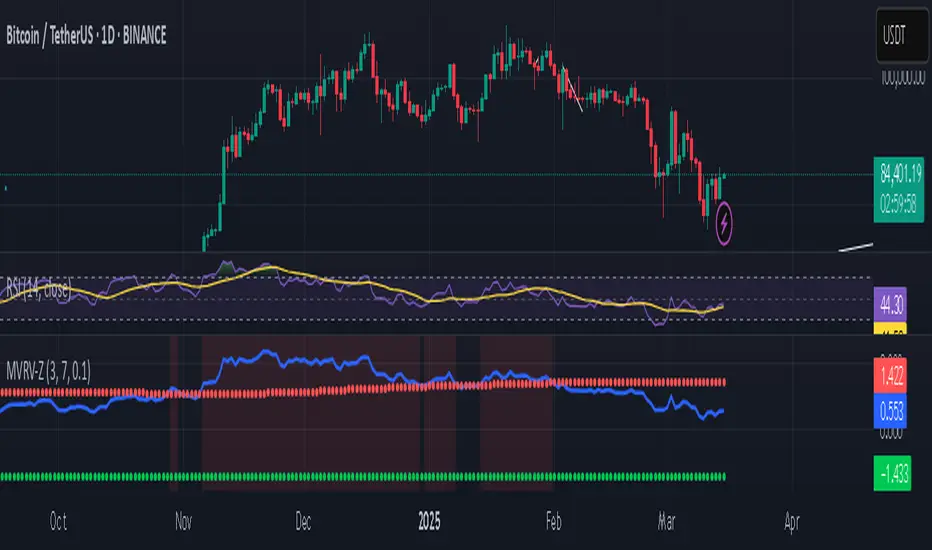
Bitcoin MVRV Z-Score Indicator### **What This Script Does (In Plain English)**
Imagine Bitcoin has a "fair price" based on what people *actually paid* for it (called the **Realized Value**). This script tells you if Bitcoin is currently **overpriced** or **underpriced** compared to that fair price, using math.
---
### **How It Works (Like a Car Dashboard)**
1. **The Speedometer (Z-Score Line)**
- The blue line (**Z-Score**) acts like a speedometer for Bitcoin’s price:
- **Above Red Line** → Bitcoin is "speeding" (overpriced).
- **Below Green Line** → Bitcoin is "parked" (underpriced).
2. **The Warning Lights (Colors)**
- **Red Background**: "Slow down!" – Bitcoin might be too expensive.
- **Green Background**: "Time to fuel up!" – Bitcoin might be a bargain.
3. **The Alarms (Alerts)**
- Your phone buzzes when:
- Green light turns on → "Buy opportunity!"
- Red light turns on → "Be careful – might be time to sell!"
---
### **Real-Life Example**
- **2021 Bitcoin Crash**:
- The red light turned on when Bitcoin hit $60,000+ (Z-Score >7).
- A few months later, Bitcoin crashed to $30,000.
- **2023 Rally**:
- The green light turned on when Bitcoin was around $20,000 (Z-Score <0.1).
- Bitcoin later rallied to $35,000.
---
### **How to Use It (3 Simple Steps)**
1. **Look at the Blue Line**:
- If it’s **rising toward the red zone**, Bitcoin is getting expensive.
- If it’s **falling toward the green zone**, Bitcoin is getting cheap.
2. **Check the Colors**:
- Trade carefully when the background is **red**.
- Look for buying chances when it’s **green**.
3. **Set Alerts**:
- Get notified when Bitcoin enters "cheap" or "expensive" zones.
---
### **Important Notes**
- **Not Magic**: This tool helps spot trends but isn’t perfect. Always combine it with other indicators.
- **Best for Bitcoin**: Works great for Bitcoin, not as well for altcoins.
- **Long-Term Focus**: Signals work best over months/years, not hours.
---
Think of it as a **thermometer for Bitcoin’s price fever** – it tells you when the market is "hot" or "cold." 🔥❄️
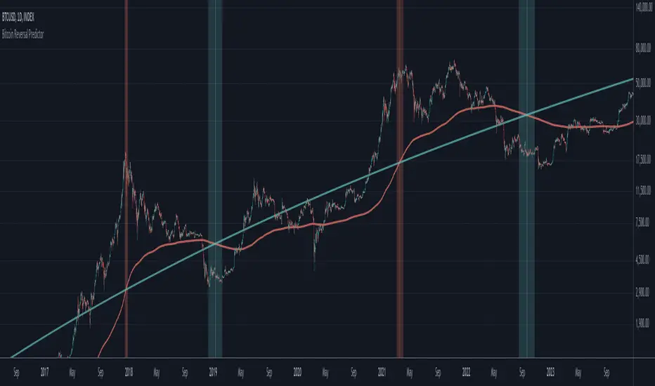
Bitcoin Reversal PredictorOverview
This indicator displays two lines that, when they cross, signal a potential reversal in Bitcoin's price trend. Historically, the high or low of a bull market cycle often occurs near the moment these lines intersect. The lines consist of an Exponential Moving Average (EMA) and a logarithmic regression line fitted to all of Bitcoin's historical data.
Inspiration
The inspiration for this indicator came from the PI Cycle Top indicator, which has accurately predicted past bull market peaks. However, I believe the PI Cycle Top indicator may not be as effective in the future. In that indicator, two lines cross to mark the top, but the extent of the cross has been diminishing over time. This was especially noticeable in the 2021 cycle, where the lines barely crossed. Because of this, I created a new indicator that I think will continue to provide reliable reversal signals in the future.
How It Works
The logarithmic regression line is fitted to the Bitcoin (BTCUSD) chart using two key factors: the 'a' factor (slope) and the 'b' factor (intercept). This results in a steadily decreasing line. The EMA oscillates above and below this regression line. Each time the two lines cross, a vertical colored bar appears, indicating that Bitcoin's price momentum is likely to reverse.
Use Cases
- Price Bottoming:
Bitcoin often bottoms out when the EMA crosses below the logarithmic regression line.
- Price Topping:
In contrast, Bitcoin often peaks when the EMA crosses above the logarithmic regression line.
- Profitable Strategy:
Trading at the crossovers of these lines can be a profitable strategy, as these moments often signal significant price reversals.
Percentages from 52 Week HighThis script is helpful for anyone that wants to monitor 5, 10, 20, 30, 40, 50% drops from the 52 week moving high.
I have been using a version of this script for a few years now and thought I would share it back with the community as I wrote it in 2021 to find quick deals when flipping through charts of stocks I've been watching. I never seemed to find anything doing this simple yet intuitive thing and I found myself regularly computing these lines manually on each chart. This will save you from having to do that as it automatically draws each level on your chart based on the recent 52 week or daily high.
I recently added the ability to turn on/off different levels and defaulted to setting 5, 10, and 20 % drops from the 52 week high. You can also change this to be a 52 day moving high if that's your preference.
Please let me know if you have ideas for modification as I wanted to share this with the community given I had not seen anything out there giving me what I wanted - which is why I wrote it.
All the best friends.

SimilarityMeasuresLibrary "SimilarityMeasures"
Similarity measures are statistical methods used to quantify the distance between different data sets
or strings. There are various types of similarity measures, including those that compare:
- data points (SSD, Euclidean, Manhattan, Minkowski, Chebyshev, Correlation, Cosine, Camberra, MAE, MSE, Lorentzian, Intersection, Penrose Shape, Meehl),
- strings (Edit(Levenshtein), Lee, Hamming, Jaro),
- probability distributions (Mahalanobis, Fidelity, Bhattacharyya, Hellinger),
- sets (Kumar Hassebrook, Jaccard, Sorensen, Chi Square).
---
These measures are used in various fields such as data analysis, machine learning, and pattern recognition. They
help to compare and analyze similarities and differences between different data sets or strings, which
can be useful for making predictions, classifications, and decisions.
---
References:
en.wikipedia.org
cran.r-project.org
numerics.mathdotnet.com
github.com
github.com
github.com
Encyclopedia of Distances, doi.org
ssd(p, q)
Sum of squared difference for N dimensions.
Parameters:
p (float ) : `array` Vector with first numeric distribution.
q (float ) : `array` Vector with second numeric distribution.
Returns: Measure of distance that calculates the squared euclidean distance.
euclidean(p, q)
Euclidean distance for N dimensions.
Parameters:
p (float ) : `array` Vector with first numeric distribution.
q (float ) : `array` Vector with second numeric distribution.
Returns: Measure of distance that calculates the straight-line (or Euclidean).
manhattan(p, q)
Manhattan distance for N dimensions.
Parameters:
p (float ) : `array` Vector with first numeric distribution.
q (float ) : `array` Vector with second numeric distribution.
Returns: Measure of absolute differences between both points.
minkowski(p, q, p_value)
Minkowsky Distance for N dimensions.
Parameters:
p (float ) : `array` Vector with first numeric distribution.
q (float ) : `array` Vector with second numeric distribution.
p_value (float) : `float` P value, default=1.0(1: manhatan, 2: euclidean), does not support chebychev.
Returns: Measure of similarity in the normed vector space.
chebyshev(p, q)
Chebyshev distance for N dimensions.
Parameters:
p (float ) : `array` Vector with first numeric distribution.
q (float ) : `array` Vector with second numeric distribution.
Returns: Measure of maximum absolute difference.
correlation(p, q)
Correlation distance for N dimensions.
Parameters:
p (float ) : `array` Vector with first numeric distribution.
q (float ) : `array` Vector with second numeric distribution.
Returns: Measure of maximum absolute difference.
cosine(p, q)
Cosine distance between provided vectors.
Parameters:
p (float ) : `array` 1D Vector.
q (float ) : `array` 1D Vector.
Returns: The Cosine distance between vectors `p` and `q`.
---
angiogenesis.dkfz.de
camberra(p, q)
Camberra distance for N dimensions.
Parameters:
p (float ) : `array` Vector with first numeric distribution.
q (float ) : `array` Vector with second numeric distribution.
Returns: Weighted measure of absolute differences between both points.
mae(p, q)
Mean absolute error is a normalized version of the sum of absolute difference (manhattan).
Parameters:
p (float ) : `array` Vector with first numeric distribution.
q (float ) : `array` Vector with second numeric distribution.
Returns: Mean absolute error of vectors `p` and `q`.
mse(p, q)
Mean squared error is a normalized version of the sum of squared difference.
Parameters:
p (float ) : `array` Vector with first numeric distribution.
q (float ) : `array` Vector with second numeric distribution.
Returns: Mean squared error of vectors `p` and `q`.
lorentzian(p, q)
Lorentzian distance between provided vectors.
Parameters:
p (float ) : `array` Vector with first numeric distribution.
q (float ) : `array` Vector with second numeric distribution.
Returns: Lorentzian distance of vectors `p` and `q`.
---
angiogenesis.dkfz.de
intersection(p, q)
Intersection distance between provided vectors.
Parameters:
p (float ) : `array` Vector with first numeric distribution.
q (float ) : `array` Vector with second numeric distribution.
Returns: Intersection distance of vectors `p` and `q`.
---
angiogenesis.dkfz.de
penrose(p, q)
Penrose Shape distance between provided vectors.
Parameters:
p (float ) : `array` Vector with first numeric distribution.
q (float ) : `array` Vector with second numeric distribution.
Returns: Penrose shape distance of vectors `p` and `q`.
---
angiogenesis.dkfz.de
meehl(p, q)
Meehl distance between provided vectors.
Parameters:
p (float ) : `array` Vector with first numeric distribution.
q (float ) : `array` Vector with second numeric distribution.
Returns: Meehl distance of vectors `p` and `q`.
---
angiogenesis.dkfz.de
edit(x, y)
Edit (aka Levenshtein) distance for indexed strings.
Parameters:
x (int ) : `array` Indexed array.
y (int ) : `array` Indexed array.
Returns: Number of deletions, insertions, or substitutions required to transform source string into target string.
---
generated description:
The Edit distance is a measure of similarity used to compare two strings. It is defined as the minimum number of
operations (insertions, deletions, or substitutions) required to transform one string into another. The operations
are performed on the characters of the strings, and the cost of each operation depends on the specific algorithm
used.
The Edit distance is widely used in various applications such as spell checking, text similarity, and machine
translation. It can also be used for other purposes like finding the closest match between two strings or
identifying the common prefixes or suffixes between them.
---
github.com
www.red-gate.com
planetcalc.com
lee(x, y, dsize)
Distance between two indexed strings of equal length.
Parameters:
x (int ) : `array` Indexed array.
y (int ) : `array` Indexed array.
dsize (int) : `int` Dictionary size.
Returns: Distance between two strings by accounting for dictionary size.
---
www.johndcook.com
hamming(x, y)
Distance between two indexed strings of equal length.
Parameters:
x (int ) : `array` Indexed array.
y (int ) : `array` Indexed array.
Returns: Length of different components on both sequences.
---
en.wikipedia.org
jaro(x, y)
Distance between two indexed strings.
Parameters:
x (int ) : `array` Indexed array.
y (int ) : `array` Indexed array.
Returns: Measure of two strings' similarity: the higher the value, the more similar the strings are.
The score is normalized such that `0` equates to no similarities and `1` is an exact match.
---
rosettacode.org
mahalanobis(p, q, VI)
Mahalanobis distance between two vectors with population inverse covariance matrix.
Parameters:
p (float ) : `array` 1D Vector.
q (float ) : `array` 1D Vector.
VI (matrix) : `matrix` Inverse of the covariance matrix.
Returns: The mahalanobis distance between vectors `p` and `q`.
---
people.revoledu.com
stat.ethz.ch
docs.scipy.org
fidelity(p, q)
Fidelity distance between provided vectors.
Parameters:
p (float ) : `array` 1D Vector.
q (float ) : `array` 1D Vector.
Returns: The Bhattacharyya Coefficient between vectors `p` and `q`.
---
en.wikipedia.org
bhattacharyya(p, q)
Bhattacharyya distance between provided vectors.
Parameters:
p (float ) : `array` 1D Vector.
q (float ) : `array` 1D Vector.
Returns: The Bhattacharyya distance between vectors `p` and `q`.
---
en.wikipedia.org
hellinger(p, q)
Hellinger distance between provided vectors.
Parameters:
p (float ) : `array` 1D Vector.
q (float ) : `array` 1D Vector.
Returns: The hellinger distance between vectors `p` and `q`.
---
en.wikipedia.org
jamesmccaffrey.wordpress.com
kumar_hassebrook(p, q)
Kumar Hassebrook distance between provided vectors.
Parameters:
p (float ) : `array` 1D Vector.
q (float ) : `array` 1D Vector.
Returns: The Kumar Hassebrook distance between vectors `p` and `q`.
---
github.com
jaccard(p, q)
Jaccard distance between provided vectors.
Parameters:
p (float ) : `array` 1D Vector.
q (float ) : `array` 1D Vector.
Returns: The Jaccard distance between vectors `p` and `q`.
---
github.com
sorensen(p, q)
Sorensen distance between provided vectors.
Parameters:
p (float ) : `array` 1D Vector.
q (float ) : `array` 1D Vector.
Returns: The Sorensen distance between vectors `p` and `q`.
---
people.revoledu.com
chi_square(p, q, eps)
Chi Square distance between provided vectors.
Parameters:
p (float ) : `array` 1D Vector.
q (float ) : `array` 1D Vector.
eps (float)
Returns: The Chi Square distance between vectors `p` and `q`.
---
uw.pressbooks.pub
stats.stackexchange.com
www.itl.nist.gov
kulczynsky(p, q, eps)
Kulczynsky distance between provided vectors.
Parameters:
p (float ) : `array` 1D Vector.
q (float ) : `array` 1D Vector.
eps (float)
Returns: The Kulczynsky distance between vectors `p` and `q`.
---
github.com

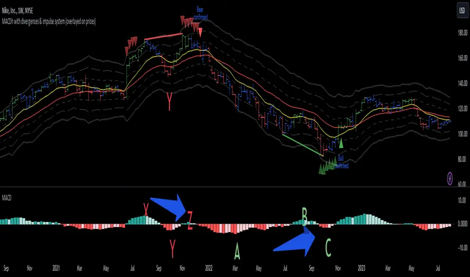
MACDh with divergences & impulse system (overlayed on prices)-----------------------------------------------------------------
General Description:
This indicator ( the one on the top panel above ) consists on some lines, arrows and labels drawn over the price bars/candles indicating the detection of regular divergences between price and the classic MACD histogram (shown on the low panel). This script is special because it can be adjusted to fit several criteria when trading divergences filtering them according to the "height" and "width" of the patterns. The script also includes the "extra features" Impulse System and Keltner Channels, which you will hardly find anywhere else in similar classic MACD histogram divergence indicators.
The indicator helps to find trend reversals, and it works on any market, any instrument, any timeframe, and any market condition (except against really strong trends that do not show any other sign of reversion yet).
Please take on consideration that divergences should be taken with caution.
-----------------------------------------------------------------
Definition of classic Bullish and Bearish divergences:
* Bearish divergences occur in uptrends identifying market tops. A classical or regular bearish divergence occurs when prices reach a new high and then pull back, with an oscillator (MACD histogram in this case) dropping below its zero line. Prices stabilize and rally to a higher high, but the oscillator reaches a lower peak than it did on a previous rally.
In the chart above (weekly charts of NKE, Nike, Inc.), in area X (around August 2021), NKE rallied to a new bull market high and MACD-Histogram rallied with it, rising above its previous peak and showing that bulls were extremely strong. In area Y, MACD-H fell below its centerline and at the same time prices punched below the zone between the two moving averages. In area Z, NKE rallied to a new bull market high, but the rally of MACD-H was feeble, reflecting the bulls’ weakness. Its downtick from peak Z completed a bearish divergence, giving a strong sell signal and auguring a nasty bear market.
* Bullish divergences , in the other hand, occur towards the ends of downtrends identifying market bottoms. A classical (also called regular) bullish divergence occurs when prices and an oscillator (MACD histogram in this case) both fall to a new low, rally, with the oscillator rising above its zero line, then both fall again. This time, prices drop to a lower low, but the oscillator traces a higher bottom than during its previous decline.
In the example in the chart above (weekly charts of NKE, Nike, Inc.), you see a bearish divergence that signaled the October 2022 bear market bottom, giving a strong buy signal right near the lows. In area A, NKE (weekly charts) appeared in a free fall. The record low A of MACD-H indicated that bears were extremely strong. In area B, MACD-H rallied above its centerline. Notice the brief rally of prices at that moment. In area C, NKE slid to a new bear market low, but MACD-H traced a much more shallow low. Its uptick completed a bullish divergence, giving a strong buy signal.
-----------------------------------------------------------------
Some cool features included in this indicator:
1. This indicator also includes the “ Impulse System ”. The Impulse System is based on two indicators, a 13-day exponential moving average and the MACD-Histogram, and identifies inflection points where a trend speeds up or slows down. The moving average identifies the trend, while the MACD-Histogram measures momentum. This unique indicator combination is color coded into the price bars for easy reference.
Calculation:
Green Price Bar: (13-period EMA > previous 13-period EMA) and
(MACD-Histogram > previous period's MACD-Histogram)
Red Price Bar: (13-period EMA < previous 13-period EMA) and
(MACD-Histogram < previous period's MACD-Histogram)
Price bars are colored blue when conditions for a Red Price Bar or Green Price Bar are not met. The MACD-Histogram is based on MACD(12,26,9).
The Impulse System works more like a censorship system. Green price bars show that the bulls are in control of both trend and momentum as both the 13-day EMA and MACD-Histogram are rising (you don't have permission to sell). A red price bar indicates that the bears have taken control because the 13-day EMA and MACD Histogram are falling (you don't have permission to buy). A blue price bar indicates mixed technical signals, with neither buying nor selling pressure predominating (either both buying or selling are permitted).
2. Another "extra feature" included here is the " Keltner Channels ". Keltner Channels are volatility-based envelopes set above and below an exponential moving average.
3. It were also included a couple of EMAs.
Everything can be removed from the chart any time.
-----------------------------------------------------------------
Options/adjustments for this indicator:
*Horizontal Distance (width) between two tops/bottoms criteria.
Refers to the horizontal distance between the MACH histogram peaks involved in the divergence
*Height of tops/bottoms criteria (for Histogram).
Refers to the difference/relation/vertical distance between the MACH HISTOGRAM peaks involved in the divergence: 1st Histogram Peak is X times the 2nd.
*Height/Vertical deviation of tops/bottoms criteria (for Price).
Deviation refers to the difference/relation/vertical distance between the PRICE peaks involved in the divergence.
*Plot Regular Bullish Divergences?.
*Plot Regular Bearish Divergences?.
*Delete Previous Cancelled Divergences?.
*Shows a pair of EMAs.
*Shows Keltner Channels (using ATR)
Keltner Channels are volatility-based envelopes set above and below an exponential moving average.
*This indicator also has the option to show the Impulse System over the price bars/candles.
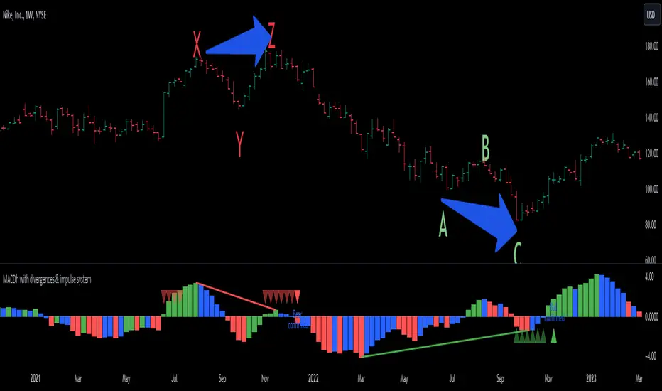
MACDh with divergences & impulse system-----------------------------------------------------------------
General Description:
This indicator ( the one on the low panel ) is a classic MACD that also shows regular divergences between its histogram and the prices. This script is special because it can be adjusted to fit several criteria when trading divergences filtering them according to the "height" and "width" of the patterns. The script also includes the "extra feature" Impulse System, which you will hardly find anywhere else in similar classic MACD histogram divergence indicators.
The indicator helps to find trend reversals, and it works on any market, any instrument, any timeframe, and any market condition (except against really strong trends that do not show any other sign of reversion yet).
Please take on consideration that divergences should be taken with caution.
-----------------------------------------------------------------
Definition of classic Bullish and Bearish divergences:
* Bearish divergences occur in uptrends identifying market tops. A classical or regular bearish divergence occurs when prices reach a new high and then pull back, with an oscillator (MACD histogram in this case) dropping below its zero line. Prices stabilize and rally to a higher high, but the oscillator reaches a lower peak than it did on a previous rally.
In the chart above (weekly charts of NKE, Nike, Inc.), in area X (around August 2021), NKE rallied to a new bull market high and MACD-Histogram rallied with it, rising above its previous peak and showing that bulls were extremely strong. In area Y, MACD-H fell below its centerline and at the same time prices punched below the zone between the two moving averages. In area Z, NKE rallied to a new bull market high, but the rally of MACD-H was feeble, reflecting the bulls’ weakness. Its downtick from peak Z completed a bearish divergence, giving a strong sell signal and auguring a nasty bear market.
* Bullish divergences , in the other hand, occur towards the ends of downtrends identifying market bottoms. A classical (also called regular) bullish divergence occurs when prices and an oscillator (MACD histogram in this case) both fall to a new low, rally, with the oscillator rising above its zero line, then both fall again. This time, prices drop to a lower low, but the oscillator traces a higher bottom than during its previous decline.
In the example in the chart above (weekly charts of NKE, Nike, Inc.), you see a bearish divergence that signaled the October 2022 bear market bottom, giving a strong buy signal right near the lows. In area A, NKE (weekly charts) appeared in a free fall. The record low A of MACD-H indicated that bears were extremely strong. In area B, MACD-H rallied above its centerline. Notice the brief rally of prices at that moment. In area C, NKE slid to a new bear market low, but MACD-H traced a much more shallow low. Its uptick completed a bullish divergence, giving a strong buy signal.
-----------------------------------------------------------------
Extra feature: Impulse System
This indicator also includes the “ Impulse System ”. The Impulse System is based on two indicators, a 13-day exponential moving average and the MACD-Histogram, and identifies inflection points where a trend speeds up or slows down. The moving average identifies the trend, while the MACD-Histogram measures momentum. This unique indicator combination is color coded into the price bars or macd histogram bars for easy reference.
Calculation:
Green Price Bar: (13-period EMA > previous 13-period EMA) and
(MACD-Histogram > previous period's MACD-Histogram)
Red Price Bar: (13-period EMA < previous 13-period EMA) and
(MACD-Histogram < previous period's MACD-Histogram)
Histogram bars are colored blue when conditions for a Red Histogram Bar or Green Histogram Bar are not met. The MACD-Histogram is based on MACD(12,26,9).
The Impulse System works more like a censorship system. Green histogram bars show that the bulls are in control of both trend and momentum as both the 13-day EMA and MACD-Histogram are rising (you don't have permission to sell). A red histogram bar indicates that the bears have taken control because the 13-day EMA and MACD Histogram are falling (you don't have permission to buy). A blue histogram bar indicates mixed technical signals, with neither buying nor selling pressure predominating (either both buying or selling are permitted).
The impulse system can be removed from the chart any time.
-----------------------------------------------------------------
Options/adjustments for this indicator:
*Horizontal Distance (width) between two tops/bottoms criteria.
Refers to the horizontal distance between the MACH histogram peaks involved in the divergence
*Height of tops/bottoms criteria (for Histogram).
Refers to the difference/relation/vertical distance between the MACH HISTOGRAM peaks involved in the divergence: 1st Histogram Peak is X times the 2nd.
*Height/Vertical deviation of tops/bottoms criteria (for Price).
Deviation refers to the difference/relation/vertical distance between the PRICE peaks involved in the divergence.
*Plot Regular Bullish Divergences?.
*Plot Regular Bearish Divergences?.
*Delete Previous Cancelled Divergences?.
*This indicator also has the option to show the Impulse System over the MACD histogram bars
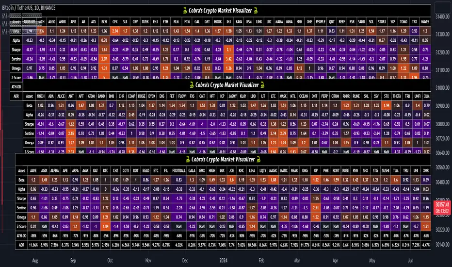
Cobra's CryptoMarket VisualizerCobra's Crypto Market Screener is designed to provide a comprehensive overview of the top 40 marketcap cryptocurrencies in a table\heatmap format. This indicator incorporates essential metrics such as Beta, Alpha, Sharpe Ratio, Sortino Ratio, Omega Ratio, Z-Score, and Average Daily Range (ADR). The table utilizes cell coloring resembling a heatmap, allowing for quick visual analysis and comparison of multiple cryptocurrencies.
The indicator also includes a shortened explanation tooltip of each metric when hovering over it's respected cell. I shall elaborate on each here for anyone interested.
Metric Descriptions:
1. Beta: measures the sensitivity of an asset's returns to the overall market returns. It indicates how much the asset's price is likely to move in relation to a benchmark index. A beta of 1 suggests the asset moves in line with the market, while a beta greater than 1 implies the asset is more volatile, and a beta less than 1 suggests lower volatility.
2. Alpha: is a measure of the excess return generated by an investment compared to its expected return, given its risk (as indicated by its beta). It assesses the performance of an investment after adjusting for market risk. Positive alpha indicates outperformance, while negative alpha suggests underperformance.
3. Sharpe Ratio: measures the risk-adjusted return of an investment or portfolio. It evaluates the excess return earned per unit of risk taken. A higher Sharpe ratio indicates better risk-adjusted performance, as it reflects a higher return for each unit of volatility or risk.
4. Sortino Ratio: is a risk-adjusted measure similar to the Sharpe ratio but focuses only on downside risk. It considers the excess return per unit of downside volatility. The Sortino ratio emphasizes the risk associated with below-target returns and is particularly useful for assessing investments with asymmetric risk profiles.
5. Omega Ratio: measures the ratio of the cumulative average positive returns to the cumulative average negative returns. It assesses the reward-to-risk ratio by considering both upside and downside performance. A higher Omega ratio indicates a higher reward relative to the risk taken.
6. Z-Score: is a statistical measure that represents the number of standard deviations a data point is from the mean of a dataset. In finance, the Z-score is commonly used to assess the financial health or risk of a company. It quantifies the distance of a company's financial ratios from the average and provides insight into its relative position.
7. Average Daily Range: ADR represents the average range of price movement of an asset during a trading day. It measures the average difference between the high and low prices over a specific period. Traders use ADR to gauge the potential price range within which an asset might fluctuate during a typical trading session.
Utility:
Comprehensive Overview: The indicator allows for monitoring up to 40 cryptocurrencies simultaneously, providing a consolidated view of essential metrics in a single table.
Efficient Comparison: The heatmap-like coloring of the cells enables easy visual comparison of different cryptocurrencies, helping identify relative strengths and weaknesses.
Risk Assessment: Metrics such as Beta, Alpha, Sharpe Ratio, Sortino Ratio, and Omega Ratio offer insights into the risk associated with each cryptocurrency, aiding risk assessment and portfolio management decisions.
Performance Evaluation: The Alpha, Sharpe Ratio, and Sortino Ratio provide measures of a cryptocurrency's performance adjusted for risk. This helps assess investment performance over time and across different assets.
Market Analysis: By considering the Z-Score and Average Daily Range (ADR), traders can evaluate the financial health and potential price volatility of cryptocurrencies, aiding in trade selection and risk management.
Features:
Reference period optimization, alpha and ADR in particular
Source calculation
Table sizing and positioning options to fit the user's screen size.
Tooltips
Important Notes -
1. The Sharpe, Sortino and Omega ratios cell coloring threshold might be subjective, I did the best I can to gauge the median value of each to provide more accurate coloring sentiment, it may change in the future.
The median values are : Sharpe -1, Sortino - 1.5, Omega - 20.
2. Limitations - Some cryptos have a Z-Score value of NaN due to their short lifetime, I tried to overcome this issue as with the rest of the metrics as best I can. Moreover, it limits the time horizon for replay mode to somewhere around Q3 of 2021 and that's with using the split option of the top half, to remain with the older cryptos.
3. For the beginner Pine enthusiasts, I recommend scimming through the script as it serves as a prime example of using key features, to name a few : Arrays, User Defined Functions, User Defined Types, For loops, Switches and Tables.
4. Beta and Alpha's benchmark instrument is BTC, due to cryptos volatility I saw no reason to use SPY or any other asset for that matter.
MA Correlation CoefficientThis script helps you visualize the correlation between the price of an asset and 4 moving averages of your choice. This indicator can help you identify trendy markets as well as trend-shifts.
Disclaimer
Bear in mind that there is always some lag when using Moving-Averages, hence the purpose of this indicator is as a trend identification tool rather than an entry-exit strategy.
Working Principle
The basic idea behind this indicator is the following:
In a trendy market you will find high correlation between price and all kinds of Moving-Averages. This works both ways, no matter bull or bear trend.
In sideways markets you might find a mix of correlations accross timeframes (2018) or high correlation with Low-Timeframe averages and low correlation with High-Timeframe averages (2021/2022).
Trend shifts might be characterised by a 'staircase' type of correlation (yellow), where the asset regains correlation with higher timeframe averages
Indicator Options
1. Source : data used for indicator calculation
1. Correlation Window : size of moving window for correlation calculation
2. Average Type :
Simple-Moving-Average (SMA)
Exponential-Moving-Average (EMA)
Hull-Moving-Average (HMA)
Volume-Weighted-Moving-Average (VWMA)
3. Lookback : number of past candles to calculate average
4. Gradient : modify gradient colors. colors relate to correlation values.
Plot Explanation
The indicator plots, using colors, the correlation of the asset with 4 averages. For every candle, 4 correlation values are generated, corresponding to 4 colors. These 4 colors are stacked one on top of the other generating the patterns explained above. These patterns may help you identify what kind of market you're in.

JS-TechTrading: VWAP Momentum_Pullback StrategyGeneral Description and Unique Features of this Script
Introducing the VWAP Momentum-Pullback Strategy (long-only) that offers several unique features:
1. Our script/strategy utilizes Mark Minervini's Trend-Template as a qualifier for identifying stocks and other financial securities in confirmed uptrends.
NOTE: In this basic version of the script, the Trend-Template has to be used as a separate indicator on TradingView (Public Trend-Template indicators are available on TradingView – community scripts). It is recommended to only execute buy signals in case the stock or financial security is in a stage 2 uptrend, which means that the criteria of the trend-template are fulfilled.
2. Our strategy is based on the supply/demand balance in the market, making it timeless and effective across all timeframes. Whether you are day trading using 1- or 5-min charts or swing-trading using daily charts, this strategy can be applied and works very well.
3. We have also integrated technical indicators such as the RSI and the MA / VWAP crossover into this strategy to identify low-risk pullback entries in the context of confirmed uptrends. By doing so, the risk profile of this strategy and drawdowns are being reduced to an absolute minimum.
Minervini’s Trend-Template and the ‘Stage-Analysis’ of the Markets
This strategy is a so-called 'long-only' strategy. This means that we only take long positions, short positions are not considered.
The best market environment for such strategies are periods of stable upward trends in the so-called stage 2 - uptrend.
In stable upward trends, we increase our market exposure and risk.
In sideways markets and downward trends or bear markets, we reduce our exposure very quickly or go 100% to cash and wait for the markets to recover and improve. This allows us to avoid major losses and drawdowns.
This simple rule gives us a significant advantage over most undisciplined traders and amateurs!
'The Trend is your Friend'. This is a very old but true quote.
What's behind it???
• 98% of stocks made their biggest gains in a Phase 2 upward trend.
• If a stock is in a stable uptrend, this is evidence that larger institutions are buying the stock sustainably.
• By focusing on stocks that are in a stable uptrend, the chances of profit are significantly increased.
• In a stable uptrend, investors know exactly what to expect from further price developments. This makes it possible to locate low-risk entry points.
The goal is not to buy at the lowest price – the goal is to buy at the right price!
Each stock goes through the same maturity cycle – it starts at stage 1 and ends at stage 4
Stage 1 – Neglect Phase – Consolidation
Stage 2 – Progressive Phase – Accumulation
Stage 3 – Topping Phase – Distribution
Stage 4 – Downtrend – Capitulation
This strategy focuses on identifying stocks in confirmed stage 2 uptrends. This in itself gives us an advantage over long-term investors and less professional traders.
By focusing on stocks in a stage 2 uptrend, we avoid losses in downtrends (stage 4) or less profitable consolidation phases (stages 1 and 3). We are fully invested and put our money to work for us, and we are fully invested when stocks are in their stage 2 uptrends.
But how can we use technical chart analysis to find stocks that are in a stable stage 2 uptrend?
Mark Minervini has developed the so-called 'trend template' for this purpose. This is an essential part of our JS-TechTrading pullback strategy. For our watchlists, only those individual values that meet the tough requirements of Minervini's trend template are eligible.
The Trend Template
• 200d MA increasing over a period of at least 1 month, better 4-5 months or longer
• 150d MA above 200d MA
• 50d MA above 150d MA and 200d MA
• Course above 50d MA, 150d MA and 200d MA
• Ideally, the 50d MA is increasing over at least 1 month
• Price at least 25% above the 52w low
• Price within 25% of 52w high
• High relative strength according to IBD.
NOTE: In this basic version of the script, the Trend-Template has to be used as a separate indicator on TradingView (Public Trend-Template indicators are available in TradingView – community scripts). It is recommended to only execute buy signals in case the stock or financial security is in a stage 2 uptrend, which means that the criteria of the trend-template are fulfilled.
This strategy can be applied to all timeframes from 5 min to daily.
The VWAP Momentum-Pullback Strateg y
For the JS-TechTrading VWAP Momentum-Pullback Strategy, only stocks and other financial instruments that meet the selected criteria of Mark Minervini's trend template are recommended for algorithmic trading with this startegy.
A further prerequisite for generating a buy signals is that the individual value is in a short-term oversold state (RSI).
When the selling pressure is over and the continuation of the uptrend can be confirmed by the MA / VWAP crossover after reaching a price low, a buy signal is issued by this strategy.
Stop-loss limits and profit targets can be set variably.
Relative Strength Index (RSI)
The Relative Strength Index (RSI) is a technical indicator developed by Welles Wilder in 1978. The RSI is used to perform a market value analysis and identify the strength of a trend as well as overbought and oversold conditions. The indicator is calculated on a scale from 0 to 100 and shows how much an asset has risen or fallen relative to its own price in recent periods.
The RSI is calculated as the ratio of average profits to average losses over a certain period of time. A high value of the RSI indicates an overbought situation, while a low value indicates an oversold situation. Typically, a value > 70 is considered an overbought threshold and a value < 30 is considered an oversold threshold. A value above 70 signals that a single value may be overvalued and a decrease in price is likely , while a value below 30 signals that a single value may be undervalued and an increase in price is likely.
For example, let's say you're watching a stock XYZ. After a prolonged falling movement, the RSI value of this stock has fallen to 26. This means that the stock is oversold and that it is time for a potential recovery. Therefore, a trader might decide to buy this stock in the hope that it will rise again soon.
The MA / VWAP Crossover Trading Strategy
This strategy combines two popular technical indicators: the Moving Average (MA) and the Volume Weighted Average Price (VWAP). The MA VWAP crossover strategy is used to identify potential trend reversals and entry/exit points in the market.
The VWAP is calculated by taking the average price of an asset for a given period, weighted by the volume traded at each price level. The MA, on the other hand, is calculated by taking the average price of an asset over a specified number of periods. When the MA crosses above the VWAP, it suggests that buying pressure is increasing, and it may be a good time to enter a long position. When the MA crosses below the VWAP, it suggests that selling pressure is increasing, and it may be a good time to exit a long position or enter a short position.
Traders typically use the MA VWAP crossover strategy in conjunction with other technical indicators and fundamental analysis to make more informed trading decisions. As with any trading strategy, it is important to carefully consider the risks and potential rewards before making any trades.
This strategy is applicable to all timeframes and the relevant parameters for the underlying indicators (RSI and MA/VWAP) can be adjusted and optimized as needed.
Backtesting
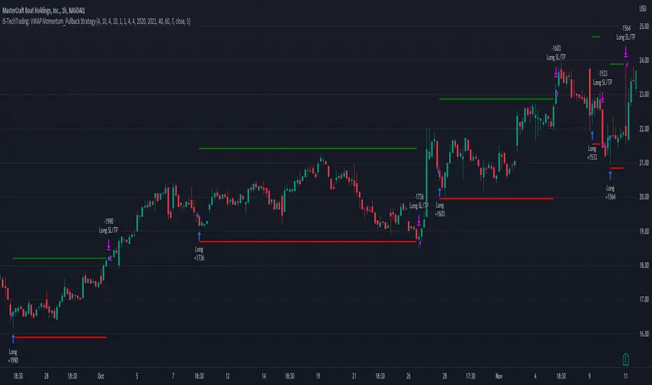
Backtesting gives outstanding results on all timeframes and drawdowns can be reduced to a minimum level. In this example, the hourly chart for MCFT has been used.
Settings for backtesting are:
- Period from April 2020 until April 2021 (1 yr)
- Starting capital 100k USD
- Position size = 25% of equity
- 0.01% commission = USD 2.50.- per Trade
- Slippage = 2 ticks
Other comments
• This strategy has been designed to identify the most promising, highest probability entries and trades for each stock or other financial security.
• The RSI qualifier is highly selective and filters out the most promising swing-trading entries. As a result, you will normally only find a low number of trades for each stock or other financial security per year in case you apply this strategy for the daily charts. Shorter timeframes will result in a higher number of trades / year.
• As a result, traders need to apply this strategy for a full watchlist rather than just one financial security.
Momentum Traffic LightScript was first published 30 May 2021 on twitter by @lehlutz
This script visualizes long, short and neutral phases of any asset class as follows:
The differences A, B, C are formed from 3 moving averages
(3-EMA exponential moving average, 20-SMA simple moving average and 50-SMA simple moving average)
namely
A: (3-EMA minus 20-SMA)
B: (3-EMA minus 50-SMA)
C: (20-SMA minus 50-SMA).
Then the following rules apply to the traffic light (where ∂ means slope).
green traffic light (bullish): (A>0,B>0,C>0), (A>0,B>0,∂C>0), (A>0,∂B>0,C>0) or (A>0,∂B>0,∂C>0, whereas ∂A>0)
red traffic light (bearish): (A<0,B<0,C<0, whereas at least ∂A or ∂B or ∂C is <0) or (A<0,B<0,∂C<0 whereas ∂A and ∂B<0);
yellow traffic light (neutral): all other
Indicator should not be considered as financial advice

Reinforced RSI - The Quant Science This strategy was designed and written with the goal of showing and motivating the community how to integrate our 'Probabilities' module with their own script.
We have recreated one of the simplest strategies used by many traders. The strategy only trades long and uses the overbought and oversold levels on the RSI indicator.
We added stop losses and take profits to offer more dynamism to the strategy. Then the 'Probabilities' module was integrated to create a probabilistic reinforcement on each trade.
Specifically, each trade is executed, only if the past probabilities of making a profitable trade is greater than or equal to 51%. This greatly increased the performance of the strategy by avoiding possible bad trades.
The backtesting was calculated on the NASDAQ:TSLA , on 15 minutes timeframe.
The strategy works on Tesla using the following parameters:
1. Lenght: 13
2. Oversold: 40
3. Overbought: 70
4. Lookback: 50
5. Take profit: 3%
6. Stop loss: 3%
Time period: January 2021 to date.
Our Probabilities Module, used in the strategy example:

Market Breadth: Trends & BreakoutsVisualize the percentage of stocks in an index participating in trends and breakouts/breakdowns.
The default data source is the S & P 500: the percent of stocks above/below the 200 and 50 day moving averages, and the percentage of stocks making new 52 week breakouts/breakdowns. You can pick new data sources in the settings.
The blue band represents the percentage of stocks above/below the 200 day moving average. (It's always 100% in width, unlike say Bollinger bands). The thin blue lines are the same but for the 50 day moving average. The red and green areas represent the percentage of stocks making new 52 week highs/lows.
In the example chart you can see a divergence between the market as a whole which continues up and to the right throughout 2021, where as fewer and fewer stocks were above their own 200 day moving average, causing the blue band to trend down. Before the market turns beginning 2022 you can see more stocks making new 52 week lows, even as other stocks make 52 week highs. After the market tops, the percentage of 52 week lows intensifies and the percentage of stocks below their 200 day moving average is already over 50%.

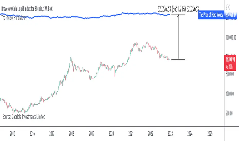
The Price of Hard MoneyIf we calculate “the price of hard money” (the market capitalization weighted price of gold plus Bitcoin); we get this chart.
Since 2017, Bitcoin’s share of hard money growth has been increasing, we can see it visibly on the gold chart by a widening delta between the price of hard money and the Gold price. We can also see some interesting technical behaviours.
In 2021, Hard Money broke out and held this breakout above the 2011 Gold high. Only later in 2022 did a correction of 20% occur – typical of Golds historic volatility in periods of inflation and high interest rates.
Hard Money is at major support and we have evidence for a fundamental shift in investor capital flows away from gold and into Bitcoin.
This Indicator is useful:
- To track the market capitalization of Gold (estimated), Bitcoin and combined market capitalization of Hard Money.
- To track the price action and respective change in investor flows from Gold to Bitcoin .
Provided Bitcoin continues to suck more value out of gold with time, this chart will be useful for tracking price action of the combined asset classes into the years to come.
Day Trading Booster by DGTTiming when day trading can be everything
In Stock markets typically more volatility (or price activity) occurs at market opening and closings
When it comes to Forex (foreign exchange market), the world’s most traded market, unlike other financial markets, there is no centralized marketplace, currencies trade over the counter in whatever market is open at that time, where time becomes of more importance and key to get better trading opportunities. There are four major forex trading sessions, which are Sydney , Tokyo , London and New York sessions
Forex market is traded 24 hours a day, 5 days a week across by banks, institutions and individual traders worldwide, but that doesn’t mean it’s always active the entire day. It may be very difficult time trying to make money when the market doesn’t move at all. The busiest times with highest trading volume occurs during the overlap of the London and New York trading sessions, because U.S. dollar (USD) and the Euro (EUR) are the two most popular currencies traded. Typically most of the trading activity for a specific currency pair will occur when the trading sessions of the individual currencies overlap. For example, Australian Dollar (AUD) and Japanese Yen (JPY) will experience a higher trading volume when both Sydney and Tokyo sessions are open
There is one influence that impacts Forex matkets and should not be forgotten : the release of the significant news and reports. When a major announcement is made regarding economic data, currency can lose or gain value within a matter of seconds
Cryptocurrency markets on the other hand remain open 24/7, even during public holidays
Until 2021, the Asian impact was so significant in Cryptocurrency markets but recent reasearch reports shows that those patterns have changed and the correlation with the U.S. trading hours is becoming a clear evolving trend.
Unlike any other market Crypto doesn’t rest on weekends, there’s a drop-off in participation and yet algorithmic trading bots and market makers (or liquidity providers) can create a high volume of activity. Never trust the weekend’ is a good thing to remind yourself
One more factor that needs to be taken into accout is Blockchain transaction fees, which are responsive to network congestion and can change dramatically from one hour to the next
In general, Cryptocurrency markets are highly volatile, which means that the price of a coin can change dramatically over a short time period in either direction
The Bottom Line
The more traders trading, the higher the trading volume, and the more active the market. The more active the market, the higher the liquidity (availability of counterparties at any given time to exit or enter a trade), hence the tighter the spreads (the difference between ask and bid price) and the less slippage (the difference between the expected fill price and the actual fill price) - in a nutshell, yield to many good trading opportunities and better order execution (a process of filling the requested buy or sell order)
The best time to trade is when the market is the most active and therefore has the largest trading volume, trading all day long will not only deplete a trader's reserves quickly, but it can burn out even the most persistent trader. Knowing when the markets are more active will give traders peace of mind, that opportunities are not slipping away when they take their eyes off the markets or need to get a few hours of sleep
What does the Day Trading Booster do?
Day Trading Booster is designed ;
- to assist in determining market peak times, the times where better trading opportunities may arise
- to assist in determining the probable trading opportunities
- to help traders create their own strategies. An example strategy of when to trade or not is presented below
For Forex markets specifically includes
- Opening channel of Asian session, Europien session or both
- Opening price, opening range (5m or 15m) and day (session) range of the major trading center sessions, including Frankfurt
- A tabular view of the major forex markets oppening/closing hours, with a countdown timer
- A graphical presentation of typically traded volume and various forext markets oppening/clossing events (not only the major markets but many other around the world)
For All type of markets Day Trading Booster plots
- Day (Session) Open, 5m, 15m or 1h Opening Range
- Day (Session) Referance Levels, based on Average True Range (ATR) or Previous Day (Session) Range (PH - PL)
- Week and Month Open
Day Trading Booster also includes some of the day trader's preffered indicaotrs, such as ;
- VWAP - A custom interpretaion of VWAP is presented here with Auto, Interactive and Manual anchoring options.
- Pivot High/Low detection - Another custom interpretation of Pivot Points High Low indicator.
- A Moving Average with option to choose among SMA, EMA, WMA and HMA
An example strategy - Channel Bearkout Strategy
When day trading a trader usually monitors/analyzes lower timeframe charts and from time to time may loose insight of what really happens on the market from higher time porspective. Do not to forget to look at the larger time frame (than the one chosen to trade with) which gives the bigger picture of market price movements and thus helps to clearly define the trend
Disclaimer : Trading success is all about following your trading strategy and the indicators should fit within your trading strategy, and not to be traded upon solely
The script is for informational and educational purposes only. Use of the script does not constitutes professional and/or financial advice. You alone the sole responsibility of evaluating the script output and risks associated with the use of the script. In exchange for using the script, you agree not to hold dgtrd TradingView user liable for any possible claim for damages arising from any decision you make based on use of the script

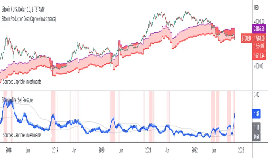
Bitcoin Miner Sell PressureBitcoin miners are in pain and now (November 2022) selling more than they have in almost 5 years!
Introducing: Bitcoin Miner Sell Pressure.
A free, open-source indicator which tracks on-chain data to highlight when Bitcoin miners are selling more of their reserves than usual.
The indicator tracks the ratio of on-chain miner Bitcoin outflows to miner Bitcoin reserves.
- Higher = more selling than usual
- Lower = less selling than usual
- Red = extraordinary sell pressure
Today , it's red.
What can we see now ?
Miners are not great at treasury management. They tend to sell most when they are losing money (like today). But there have been times when they sold well into high profit, such as into the 2017 $20K top and in early 2021 when Bitcoin breached $40K.
Bitcoin Miner Sell Pressure identifies industry stress, excess and miner capitulation.
Unsurprisingly, there is a high correlation with Bitcoin Production Cost; giving strong confluence to both.
In some instances, BMSP spots capitulation before Hash Ribbons. Such as today!
NetLiquidityLibraryLibrary "NetLiquidityLibrary"
The Net Liquidity Library provides daily values for net liquidity. Net liquidity is measured as Fed Balance Sheet - Treasury General Account - Reverse Repo. Time series for each individual component included too.
get_net_liquidity_for_date(t)
Function takes date in timestamp form and returns the Net Liquidity value for that date. If date is not present, 0 is returned.
Parameters:
t : The timestamp of the date you are requesting the Net Liquidity value for.
Returns: The Net Liquidity value for the specified date.
get_net_liquidity()
Gets the Net Liquidity time series from Dec. 2021 to current. Dates that are not present are represented as 0.
Returns: The Net Liquidity time series.

YOY[TV1]Year-to-year comparison is a popular and effective way to evaluate a company's financial performance and investment performance.
Any measurable event that repeats yearly can be compared based on YoY.
As a rule, the indicator YoY (year to year) is the number of percentages indicating an increase or regression in relation to the future or past period.
For example, you can compare WM2NS using the YOY (Year to Year) method.
The Offset argument sets the data comparison period. For daily, weekly and monthly timeframes, if Offset is set to 0, it will be determined automatically.
Сравнение Год к году - популярный и эффективный способ оценки финансовых показателей компании и эффективность инвестиций.
Любое измеримое событие, которое повторяется ежегодно можно сравнить на основе YoY.
Как правило, показателем YoY (year to year) является количество процентов указывающее на прирост или регресс по отношению к будущему или прошлому периоду.
Например, вы можете сравнить WM2NS (эмиссию доллара) с помощью метода YOY (Год к году).
Допустим, в 2021 году вы эмитировали А долларов, а в 2022 вы эмитировали Б долларов
Итак итоговой формулой будет: ((Б - А) / А) * 100
Аргумент Offset устанавливает период сравнения данных. Для дневного, недельного и месячного таймфрейма, если Offset установлен в 0, будет определен автоматически.

RSI Past Can Turn RSI Into a Directional ToolThe Relative Strength Index was created by J. Welles Wilder to measure overbought and oversold conditions. It’s also found popularity as an overall measure of direction because upward-trending stocks often hit overbought conditions. The opposite can be true with underperformers.
Today’s custom script, RSI Past, attempts to capture this secondary use of RSI as a directional indicator.
RSI Past achieves this by comparing how many bars have passed since RSI's most recent overbought and oversold readings. It then plots a simple difference between those two numbers.
Stocks with “bullish” signals will have positive readings that will increase each time RSI hits an overbought condition.
“Bearish” readings are just the opposite, growing more negative as oversold conditions occur.
An examination of some individual stocks may show the usefulness of this approach.
Meta Platforms , for example, hit an oversold condition almost exactly one year ago, and has remained under heavy selling pressure since:
Exxon Mobil , on the other hand, flipped to a bullish reading last October and has trended higher since:
This raises some interesting questions for Apple, shown on the main chart above. AAPL’s RSI Past has maintained a bullish reading for over a year -- unlike most other big technology stocks and the broader Nasdaq-100. Could this reflect bigger directional strength, especially with prices holding the $150 level that’s had relevance several times mid-2021?
TradeStation has, for decades, advanced the trading industry, providing access to stocks, options, futures and cryptocurrencies. See our Overview for more.
Important Information
TradeStation Securities, Inc., TradeStation Crypto, Inc., and TradeStation Technologies, Inc. are each wholly owned subsidiaries of TradeStation Group, Inc., all operating, and providing products and services, under the TradeStation brand and trademark. You Can Trade, Inc. is also a wholly owned subsidiary of TradeStation Group, Inc., operating under its own brand and trademarks. TradeStation Crypto, Inc. offers to self-directed investors and traders cryptocurrency brokerage services. It is neither licensed with the SEC or the CFTC nor is it a Member of NFA. When applying for, or purchasing, accounts, subscriptions, products, and services, it is important that you know which company you will be dealing with. Please click here for further important information explaining what this means.
This content is for informational and educational purposes only. This is not a recommendation regarding any investment or investment strategy. Any opinions expressed herein are those of the author and do not represent the views or opinions of TradeStation or any of its affiliates.
Investing involves risks. Past performance, whether actual or indicated by historical tests of strategies, is no guarantee of future performance or success. There is a possibility that you may sustain a loss equal to or greater than your entire investment regardless of which asset class you trade (equities, options, futures, or digital assets); therefore, you should not invest or risk money that you cannot afford to lose. Before trading any asset class, first read the relevant risk disclosure statements on the Important Documents page, found here: www.tradestation.com .

STD-Filtered, Variety FIR Digital Filters w/ ATR Bands [Loxx]STD-Filtered, Variety FIR Digital Filters w/ ATR Bands is a FIR Digital Filter indicator with ATR bands. This indicator contains 12 different digital filters. Some of these have already been covered by indicators that I've recently posted. The difference here is that this indicator has ATR bands, allows for frequency filtering, adds a frequency multiplier, and attempts show causality by lagging price input by 1/2 the period input during final application of weights. Period is restricted to even numbers.
The 3 most important parameters are the frequency cutoff, the filter window type and the "causal" parameter.
Included filter types:
- Hamming
- Hanning
- Blackman
- Blackman Harris
- Blackman Nutall
- Nutall
- Bartlet Zero End Points
- Bartlet Hann
- Hann
- Sine
- Lanczos
- Flat Top
Frequency cutoff can vary between 0 and 0.5. General rule is that the greater the cutoff is the "faster" the filter is, and the smaller the cutoff is the smoother the filter is.
You can read more about discrete-time signal processing and some of the windowing functions in this indicator here:
Window function
Window Functions and Their Applications in Signal Processing
What are FIR Filters?
In discrete-time signal processing, windowing is a preliminary signal shaping technique, usually applied to improve the appearance and usefulness of a subsequent Discrete Fourier Transform. Several window functions can be defined, based on a constant (rectangular window), B-splines, other polynomials, sinusoids, cosine-sums, adjustable, hybrid, and other types. The windowing operation consists of multipying the given sampled signal by the window function. For trading purposes, these FIR filters act as advanced weighted moving averages.
A finite impulse response (FIR) filter is a filter whose impulse response (or response to any finite length input) is of finite duration, because it settles to zero in finite time. This is in contrast to infinite impulse response (IIR) filters, which may have internal feedback and may continue to respond indefinitely (usually decaying).
The impulse response (that is, the output in response to a Kronecker delta input) of an Nth-order discrete-time FIR filter lasts exactly {\displaystyle N+1}N+1 samples (from first nonzero element through last nonzero element) before it then settles to zero.
FIR filters can be discrete-time or continuous-time, and digital or analog.
A FIR filter is (similar to, or) just a weighted moving average filter, where (unlike a typical equally weighted moving average filter) the weights of each delay tap are not constrained to be identical or even of the same sign. By changing various values in the array of weights (the impulse response, or time shifted and sampled version of the same), the frequency response of a FIR filter can be completely changed.
An FIR filter simply CONVOLVES the input time series (price data) with its IMPULSE RESPONSE. The impulse response is just a set of weights (or "coefficients") that multiply each data point. Then you just add up all the products and divide by the sum of the weights and that is it; e.g., for a 10-bar SMA you just add up 10 bars of price data (each multiplied by 1) and divide by 10. For a weighted-MA you add up the product of the price data with triangular-number weights and divide by the total weight.
What is a Standard Deviation Filter?
If price or output or both don't move more than the (standard deviation) * multiplier then the trend stays the previous bar trend. This will appear on the chart as "stepping" of the moving average line. This works similar to Super Trend or Parabolic SAR but is a more naive technique of filtering.
Included
Bar coloring
Loxx's Expanded Source Types
Signals
Alerts
Related indicators
STD/C-Filtered, N-Order Power-of-Cosine FIR Filter
STD/C-Filtered, Power-of-Cosine FIR Filter
STD/C-Filtered, Truncated Taylor Family FIR Filter
STD/Clutter-Filtered, Variety FIR Filters
STD/Clutter-Filtered, Kaiser Window FIR Digital Filter
Ehlers Two-Pole Predictor [Loxx]Ehlers Two-Pole Predictor is a new indicator by John Ehlers . The translation of this indicator into PineScript™ is a collaborative effort between @cheatcountry and I.
The following is an excerpt from "PREDICTION" , by John Ehlers
Niels Bohr said “Prediction is very difficult, especially if it’s about the future.”. Actually, prediction is pretty easy in the context of technical analysis . All you have to do is to assume the market will behave in the immediate future just as it has behaved in the immediate past. In this article we will explore several different techniques that put the philosophy into practice.
LINEAR EXTRAPOLATION
Linear extrapolation takes the philosophical approach quite literally. Linear extrapolation simply takes the difference of the last two bars and adds that difference to the value of the last bar to form the prediction for the next bar. The prediction is extended further into the future by taking the last predicted value as real data and repeating the process of adding the most recent difference to it. The process can be repeated over and over to extend the prediction even further.
Linear extrapolation is an FIR filter, meaning it depends only on the data input rather than on a previously computed value. Since the output of an FIR filter depends only on delayed input data, the resulting lag is somewhat like the delay of water coming out the end of a hose after it supplied at the input. Linear extrapolation has a negative group delay at the longer cycle periods of the spectrum, which means water comes out the end of the hose before it is applied at the input. Of course the analogy breaks down, but it is fun to think of it that way. As shown in Figure 1, the actual group delay varies across the spectrum. For frequency components less than .167 (i.e. a period of 6 bars) the group delay is negative, meaning the filter is predictive. However, the filter has a positive group delay for cycle components whose periods are shorter than 6 bars.
Figure 1
Here’s the practical ramification of the group delay: Suppose we are projecting the prediction 5 bars into the future. This is fine as long as the market is continued to trend up in the same direction. But, when we get a reversal, the prediction continues upward for 5 bars after the reversal. That is, the prediction fails just when you need it the most. An interesting phenomenon is that, regardless of how far the extrapolation extends into the future, the prediction will always cross the signal at the same spot along the time axis. The result is that the prediction will have an overshoot. The amplitude of the overshoot is a function of how far the extrapolation has been carried into the future.
But the overshoot gives us an opportunity to make a useful prediction at the cyclic turning point of band limited signals (i.e. oscillators having a zero mean). If we reduce the overshoot by reducing the gain of the prediction, we then also move the crossing of the prediction and the original signal into the future. Since the group delay varies across the spectrum, the effect will be less effective for the shorter cycles in the data. Nonetheless, the technique is effective for both discretionary trading and automated trading in the majority of cases.
EXPLORING THE CODE
Before we predict, we need to create a band limited indicator from which to make the prediction. I have selected a “roofing filter” consisting of a High Pass Filter followed by a Low Pass Filter. The tunable parameter of the High Pass Filter is HPPeriod. Think of it as a “stone wall filter” where cycle period components longer than HPPeriod are completely rejected and cycle period components shorter than HPPeriod are passed without attenuation. If HPPeriod is set to be a large number (e.g. 250) the indicator will tend to look more like a trending indicator. If HPPeriod is set to be a smaller number (e.g. 20) the indicator will look more like a cycling indicator. The Low Pass Filter is a Hann Windowed FIR filter whose tunable parameter is LPPeriod. Think of it as a “stone wall filter” where cycle period components shorter than LPPeriod are completely rejected and cycle period components longer than LPPeriod are passed without attenuation. The purpose of the Low Pass filter is to smooth the signal. Thus, the combination of these two filters forms a “roofing filter”, named Filt, that passes spectrum components between LPPeriod and HPPeriod.
Since working into the future is not allowed in EasyLanguage variables, we need to convert the Filt variable to the data array XX. The data array is first filled with real data out to “Length”. I selected Length = 10 simply to have a convenient starting point for the prediction. The next block of code is the prediction into the future. It is easiest to understand if we consider the case where count = 0. Then, in English, the next value of the data array is equal to the current value of the data array plus the difference between the current value and the previous value. That makes the prediction one bar into the future. The process is repeated for each value of count until predictions up to 10 bars in the future are contained in the data array. Next, the selected prediction is converted from the data array to the variable “Prediction”. Filt is plotted in Red and Prediction is plotted in yellow.
The Predict Extrapolation indicator is shown below for the Emini S&P Futures contract using the default input parameters. Filt is plotted in red and Predict is plotted in yellow. The crossings of the Predict and Filt lines provide reliable buy and sell timing signals. There is some overshoot for the shorter cycle periods, for example in February and March 2021, but the only effect is a late timing signal. Further reducing the gain and/or reducing the BarsFwd inputs would provide better timing signals during this period.
Figure 2. Predict Extrapolation Provides Reliable Timing Signals
I have experimented with other FIR filters for predictions, but found none that had a significant advantage over linear extrapolation.
MESA
MESA is an acronym for Maximum Entropy Spectral Analysis. Conceptually, it removes spectral components until the residual is left with maximum entropy. It does this by forming an all-pole filter whose order is determined by the selected number of coefficients. It maximally addresses the data within the selected window and ignores all other data. Its resolution is determined only by the number of filter coefficients selected. Since the resulting filter is an IIR filter, a prediction can be formed simply by convolving the filter coefficients with the data. MESA is one of the few, if not the only way to practically determine the coefficients of a higher order IIR filter. Discussion of MESA is beyond the scope of this article.
TWO POLE IIR FILTER
While the coefficients of a higher order IIR filter are difficult to compute without MESA, it is a relatively simple matter to compute the coefficients of a two pole IIR filter.
(Skip this paragraph if you don’t care about DSP) We can locate the conjugate pole positions parametrically in the Z plane in polar coordinates. Let the radius be QQ and the principal angle be 360 / P2Period. The first order component is 2*QQ*Cosine(360 / P2Period) and the second order component is just QQ2. Therefore, the transfer response becomes:
H(z) = 1 / (1 - 2*QQ*Cosine(360 / P2Period)*Z-1 + QQ2*Z-2)
By mixing notation we can easily convert the transfer response to code.
Output / Input = 1 / (1 - 2*QQ*Cosine(360 / P2Period)* + QQ2* )
Output - 2*QQ*Cosine(360 / P2Period)*Output + QQ2*Output = Input
Output = Input + 2*QQ*Cosine(360 / P2Period)*Output - QQ2*Output
The Two Pole Predictor starts by computing the same “roofing filter” design as described for the Linear Extrapolation Predictor. The HPPeriod and LPPeriod inputs adjust the roofing filter to obtain the desired appearance of an indicator. Since EasyLanguage variables cannot be extended into the future, the prediction process starts by loading the XX data array with indicator data up to the value of Length. I selected Length = 10 simply to have a convenient place from which to start the prediction. The coefficients are computed parametrically from the conjugate pole positions and are normalized to their sum so the IIR filter will have unity gain at zero frequency.
The prediction is formed by convolving the IIR filter coefficients with the historical data. It is easiest to see for the case where count = 0. This is the initial prediction. In this case the new value of the XX array is formed by successively summing the product of each filter coefficient with its respective historical data sample. This process is significantly different from linear extrapolation because second order curvature is introduced into the prediction rather than being strictly linear. Further, the prediction is adaptive to market conditions because the degree of curvature depends on recent historical data. The prediction in the data array is converted to a variable by selecting the BarsFwd value. The prediction is then plotted in yellow, and is compared to the indicator plotted in red.
The Predict 2 Pole indicator is shown above being applied to the Emini S&P Futures contract for most of 2021. The default parameters for the roofing filter and predictor were used. By comparison to the Linear Extrapolation prediction of Figure 2, the Predict 2 Pole indicator has a more consistent prediction. For example, there is little or no overshoot in February or March while still giving good predictions in April and May.
Input parameters can be varied to adjust the appearance of the prediction. You will find that the indicator is relatively insensitive to the BarsFwd input. The P2Period parameter primarily controls the gain of the prediction and the QQ parameter primarily controls the amount of prediction lead during trending sections of the indicator.
TAKEAWAYS
1. A more or less universal band limited “roofing filter” indicator was used to demonstrate the predictors. The HPPeriod input parameter is used to control whether the indicator looks more like a trend indicator or more like a cycle indicator. The LPPeriod input parameter is used to control the smoothness of the indicator.
2. A linear extrapolation predictor is formed by adding the difference of the two most recent data bars to the value of the last data bar. The result is considered to be a real data point and the process is repeated to extend the prediction into the future. This is an FIR filter having a one bar negative group delay at zero frequency, but the group delay is not constant across the spectrum. This variable group delay causes the linear extrapolation prediction to be inconsistent across a range of market conditions.
3. The degree of prediction by linear extrapolation can be controlled by varying the gain of the prediction to reduce the overshoot to be about the same amplitude as the peak swing of the indicator.
4. I was unable to experimentally derive a higher order FIR filter predictor that had advantages over the simple linear extrapolation predictor.
5. A Two Pole IIR predictor can be created by parametrically locating the conjugate pole positions.
6. The Two Pole predictor is a second order filter, which allows curvature into the prediction, thus mitigating overshoot. Further, the curvature is adaptive because the prediction depends on previously computed prediction values.
7. The Two Pole predictor is more consistent over a range of market conditions.
ADDITIONS
Loxx's Expanded source types:
Library for expanded source types:
Explanation for expanded source types:
Three different signal types: 1) Prediction/Filter crosses; 2) Prediction middle crosses; and, 3) Filter middle crosses.
Bar coloring to color trend.
Signals, both Long and Short.
Alerts, both Long and Short.
