Wyszukaj w skryptach "2014年日元兑美元平均汇率"
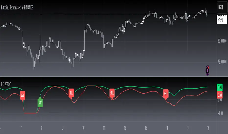
Williams Vix Fix ultra complete indicator (Tartigradia)Williams VixFix is a realized volatility indicator developed by Larry Williams, and can help in finding market bottoms.
Indeed, as Williams describe in his paper, markets tend to find the lowest prices during times of highest volatility, which usually accompany times of highest fear. The VixFix is calculated as how much the current low price statistically deviates from the maximum within a given look-back period.
Although the VixFix originally only indicates market bottoms, its inverse may indicate market tops. As masa_crypto writes : "The inverse can be formulated by considering "how much the current high value statistically deviates from the minimum within a given look-back period." This transformation equates Vix_Fix_inverse. This indicator can be used for finding market tops, and therefore, is a good signal for a timing for taking a short position." However, in practice, the Inverse VixFix is much less reliable than the classical VixFix, but is nevertheless a good addition to get some additional context.
For more information on the Vix Fix, which is a strategy published under public domain:
* The VIX Fix, Larry Williams, Active Trader magazine, December 2007, web.archive.org
* Fixing the VIX: An Indicator to Beat Fear, Amber Hestla-Barnhart, Journal of Technical Analysis, March 13, 2015, ssrn.com
* Replicating the CBOE VIX using a synthetic volatility index trading algorithm, Dayne Cary and Gary van Vuuren, Cogent Economics & Finance, Volume 7, 2019, Issue 1, doi.org
Created By ChrisMoody on 12-26-2014...
V3 MAJOR Update on 1-05-2014
tista merged LazyBear's Black Dots filter in 2020:
Extended by Tartigradia in 10-2022:
* Can select a symbol different from current to calculate vixfix, allows to select SP:SPX to mimic the original VIX index.
* Inverse VixFix (from masa_crypto and web.archive.org)
* VixFix OHLC Bars plot
* Price / VixFix Candles plot (Pro Tip: draw trend lines to find good entry/exit points)
* Add ADX filtering, Minimaxis signals, Minimaxis filtering (from samgozman )
* Convert to pinescript v5
* Allow timeframe selection (MTF)
* Skip off days (more accurate reproduction of original VIX)
* Reorganized, cleaned up code, commented out parts, commented out or removed unused code (eg, some of the KC calculations)
* Changed default Bollinger Band settings to reduce false positives in crypto markets.
Set Index symbol to SPX, and index_current = false, and timeframe Weekly, to reproduce the original VIX as close as possible by the VIXFIX (use the Add Symbol option, because you want to plot CBOE:VIX on the same timeframe as the current chart, which may include extended session / weekends). With the Weekly timeframe, off days / extended session days should not change much, but with lower timeframes this is important, because nights and weekends can change how the graph appears and seemingly make them different because of timing misalignment when in reality they are not when properly aligned.

BTC Bear Market Identifier [ChuckBanger]I have never find a use case for Line Break chart before. But I stumbled on the fact that if bitcoin dumps below the low of a big down move. It is very likely Bitcoin is heading for a new bear market. So this script is based on that idea and developed to this. It is intended to be used as a bear market identifier only with Line Break daily or higher time frame chart. If someone find a different use case for this script let me know
2014:
2018:

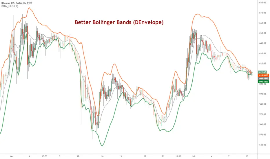
DEnvelope [Better Bollinger Bands]*** ***
Bollinger Bands (BB) usually expand quickly after a volatility increase but contract more slowly as volatility declines. This extended time it takes for BB to contract after a volatility drop can make trading some instruments using BB alone difficult or less profitable.
In the October 1998 issue of "Futures" there is an article written by Dennis McNicholl called "Better Bollinger Bands", in which the author recommends improving BB by modifying:
- the center line formula &
- different equations for calculating the bands.
These bands, called "DEnvelope", follow price more closely and respond faster to changes in volatility with these modifications.
Fore more indicators, check out my "Master Index of indicators" (Also check my published charts page for new ones I haven't added to that list):
More scripts related to DEnvelope:
------------------------------------------------
- DEnvelope Bandwidth: pastebin.com
- DEnvelope %B : pastebin.com
Sample chart with above indicators: www.tradingview.com
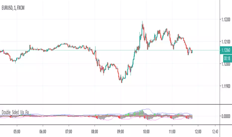
Double Sided Vix FixVixFix Enhanced by PeterO - Inverse Vix_Fix added, so now this is a dual-sided script (original VixFix shows only lows)
Note from the author: I wouldn't advise betting your strategies entirely on VixFix concept.
Original VixFix created by ChrisMoody on 12-26-2014...V3 MAJOR Update on 1-05-2014
[blackcat] L2 Ehlers Super Smoother FilterLevel: 2
Background
John F. Ehlers introuced Super Smoother Filter in Jan, 2014.
Function
In “Predictive And Successful Indicators” in Jan, 2014, John Ehlers describes a new method for smoothing market data while reducing the lag that most other smoothing techniques have. And this is a very popular filter to eliminate noise of market signal.
Key Signal
Filt --> Ehlers Super Smoother Filter fast line
Trigger --> Ehlers Super Smoother Filter slow line
Pros and Cons
100% John F. Ehlers definition translation, even variable names are the same. This help readers who would like to use pine to read his book.
Remarks
The 100th script for Blackcat1402 John F. Ehlers Week publication.
Readme
In real life, I am a prolific inventor. I have successfully applied for more than 60 international and regional patents in the past 12 years. But in the past two years or so, I have tried to transfer my creativity to the development of trading strategies. Tradingview is the ideal platform for me. I am selecting and contributing some of the hundreds of scripts to publish in Tradingview community. Welcome everyone to interact with me to discuss these interesting pine scripts.
The scripts posted are categorized into 5 levels according to my efforts or manhours put into these works.
Level 1 : interesting script snippets or distinctive improvement from classic indicators or strategy. Level 1 scripts can usually appear in more complex indicators as a function module or element.
Level 2 : composite indicator/strategy. By selecting or combining several independent or dependent functions or sub indicators in proper way, the composite script exhibits a resonance phenomenon which can filter out noise or fake trading signal to enhance trading confidence level.
Level 3 : comprehensive indicator/strategy. They are simple trading systems based on my strategies. They are commonly containing several or all of entry signal, close signal, stop loss, take profit, re-entry, risk management, and position sizing techniques. Even some interesting fundamental and mass psychological aspects are incorporated.
Level 4 : script snippets or functions that do not disclose source code. Interesting element that can reveal market laws and work as raw material for indicators and strategies. If you find Level 1~2 scripts are helpful, Level 4 is a private version that took me far more efforts to develop.
Level 5 : indicator/strategy that do not disclose source code. private version of Level 3 script with my accumulated script processing skills or a large number of custom functions. I had a private function library built in past two years. Level 5 scripts use many of them to achieve private trading strategy.

[blackcat] L2 Ehlers Early Onset TrendLevel: 2
Background
John F. Ehlers introuced Early Onset Trend Indicator in Aug, 2014.
Function
In “The Quotient Transform” in Aug, 2014, John Ehlers described an early trend detection method, the idea of the quotient transform, that was designed to reduce the lag often found in other trend indicators. I provided a script with pine v4 code here for the early-onset trend-detection indicator and also describes an approach for creating a strategy based on this indicator as an example.
The entry points displayed in blue on the price chart are defined by the top Onset Trend Detector upper quotient crossing above a threshold value e.g zero or 0.25/-0.25 here in this script. In the article, Ehlers suggested using a different K value for the exit, so the exit points are determined by the lower Onset Trend Detector quotient crossing below a threshold e.g. zero or -0.25/0.25 here in this script.
Key Signal
Quotient1 --> upper quotient in yellow which determines long entry
Quotient2 --> lower quotient in fuchsia which determines short entry
long ---> long entry signal
short ---> short entry signal
Pros and Cons
100% John F. Ehlers definition translation, even variable names are the same. This help readers who would like to use pine to read his book.
Remarks
The 82th script for Blackcat1402 John F. Ehlers Week publication.
Readme
In real life, I am a prolific inventor. I have successfully applied for more than 60 international and regional patents in the past 12 years. But in the past two years or so, I have tried to transfer my creativity to the development of trading strategies. Tradingview is the ideal platform for me. I am selecting and contributing some of the hundreds of scripts to publish in Tradingview community. Welcome everyone to interact with me to discuss these interesting pine scripts.
The scripts posted are categorized into 5 levels according to my efforts or manhours put into these works.
Level 1 : interesting script snippets or distinctive improvement from classic indicators or strategy. Level 1 scripts can usually appear in more complex indicators as a function module or element.
Level 2 : composite indicator/strategy. By selecting or combining several independent or dependent functions or sub indicators in proper way, the composite script exhibits a resonance phenomenon which can filter out noise or fake trading signal to enhance trading confidence level.
Level 3 : comprehensive indicator/strategy. They are simple trading systems based on my strategies. They are commonly containing several or all of entry signal, close signal, stop loss, take profit, re-entry, risk management, and position sizing techniques. Even some interesting fundamental and mass psychological aspects are incorporated.
Level 4 : script snippets or functions that do not disclose source code. Interesting element that can reveal market laws and work as raw material for indicators and strategies. If you find Level 1~2 scripts are helpful, Level 4 is a private version that took me far more efforts to develop.
Level 5 : indicator/strategy that do not disclose source code. private version of Level 3 script with my accumulated script processing skills or a large number of custom functions. I had a private function library built in past two years. Level 5 scripts use many of them to achieve private trading strategy.
[blackcat] L2 Ehlers Super Smooth Stoch StrategyLevel: 2
Background
John F. Ehlers introuced Super Smooth Stochastic Indicator in Jan, 2014.
Function
In “Predictive And Successful Indicators” of in, 2014, John Ehlers presented another innovative way to eliminate noise from classic indicators and introduces some new smoothing indicators: the SuperSmoother filter, which is superior to moving averages for removing aliasing noise, and the MESA Stochastic oscillator, a stochastic successor that removes the effect of spectral dilation through the use of a roofing filter.
John Ehlers described a new method for smoothing market data while reducing the lag that most other smoothing techniques have. Ehlers had provided an approach for creating a strategy. For convenience, I made the same code available at tradingview pine v4 as well as an example strategy based on Ehlers’ description. Ehlers introduced a simple countertrend system that goes long when MESA Stochastic crosses below the oversold value and reverses the trade by taking a short position when the oscillator exceeds the overbought threshold.
Key Signal
MyStochastic --> Super Smooth Stochastic line
long ---> long entry signal
short ---> short entry signal
Pros and Cons
100% John F. Ehlers definition translation, even variable names are the same. This help readers who would like to use pine to read his book.
Remarks
The 81th script for Blackcat1402 John F. Ehlers Week publication.
Readme
In real life, I am a prolific inventor. I have successfully applied for more than 60 international and regional patents in the past 12 years. But in the past two years or so, I have tried to transfer my creativity to the development of trading strategies. Tradingview is the ideal platform for me. I am selecting and contributing some of the hundreds of scripts to publish in Tradingview community. Welcome everyone to interact with me to discuss these interesting pine scripts.
The scripts posted are categorized into 5 levels according to my efforts or manhours put into these works.
Level 1 : interesting script snippets or distinctive improvement from classic indicators or strategy. Level 1 scripts can usually appear in more complex indicators as a function module or element.
Level 2 : composite indicator/strategy. By selecting or combining several independent or dependent functions or sub indicators in proper way, the composite script exhibits a resonance phenomenon which can filter out noise or fake trading signal to enhance trading confidence level.
Level 3 : comprehensive indicator/strategy. They are simple trading systems based on my strategies. They are commonly containing several or all of entry signal, close signal, stop loss, take profit, re-entry, risk management, and position sizing techniques. Even some interesting fundamental and mass psychological aspects are incorporated.
Level 4 : script snippets or functions that do not disclose source code. Interesting element that can reveal market laws and work as raw material for indicators and strategies. If you find Level 1~2 scripts are helpful, Level 4 is a private version that took me far more efforts to develop.
Level 5 : indicator/strategy that do not disclose source code. private version of Level 3 script with my accumulated script processing skills or a large number of custom functions. I had a private function library built in past two years. Level 5 scripts use many of them to achieve private trading strategy.

Mayer Multiple v2.0 - Klahr ThresholdThis is a simple update to the Mayer Multiple script by Unbound , which charts an indicator created by Trace Mayer and popularized by Preston Pysh.
The original post identified any price below 2.4x the 100-day MA as the BTC buy threshold. While the logic there is historically sound, it does not account for the fact that the BTC trend is parabolic in nature. With that in mind, I've attempted to update the 2.4x multiple to react based on the moving average of the Mayer Multiple itself. To do so, I simply found the number that, when added to the MM moving average, historically hit the 2.4x multiple during periods of low volatility. This turns out to be 1.17.
The green line represents the Klahr Threshold (is it obnoxious if I call it that? I've always wanted an indicator named after me). As you can see from the above chart, it hovers around 2.4x in late 2012 to early 2013, rises above it until mid 2014, and then stays below until 2016. It then stays almost exactly at 2.4x until April 2017, when it rises significantly above it for the first time since July 2014. The convergence in late 2012 and 2016-2017 is what leads me to believe that this should be the basis for the updated threshold.
It's entirely possible that there's a more robust method of calculating a reactive threshold (or a different number that should be added to the multiple's MA), but I think this is a good first step in refining the multiple to withstand the test of time.

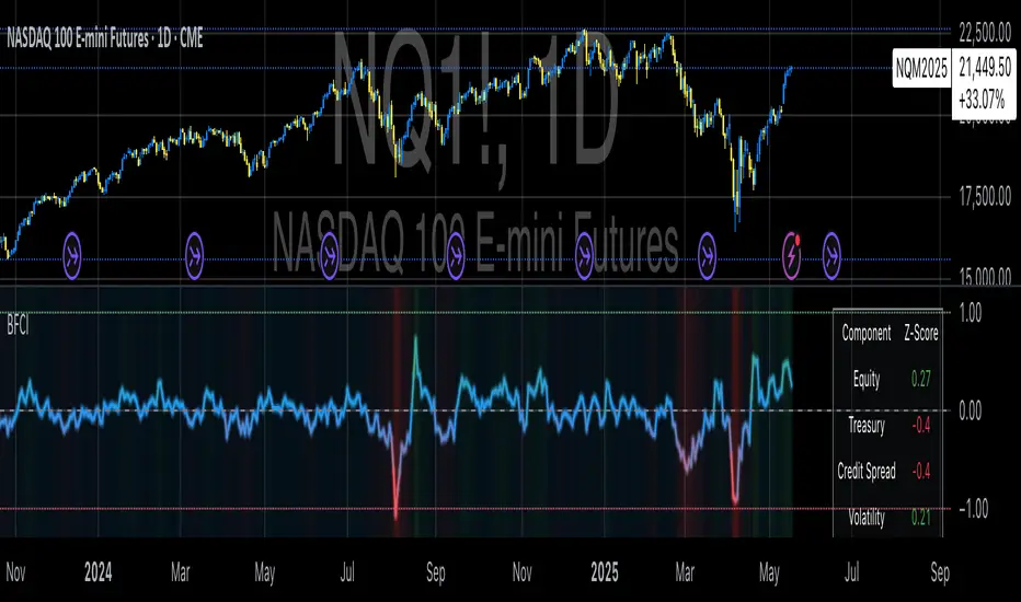
Bloomberg Financial Conditions Index (Proxy)The Bloomberg Financial Conditions Index (BFCI): A Proxy Implementation
Financial conditions indices (FCIs) have become essential tools for economists, policymakers, and market participants seeking to quantify and monitor the overall state of financial markets. Among these measures, the Bloomberg Financial Conditions Index (BFCI) has emerged as a particularly influential metric. Originally developed by Bloomberg L.P., the BFCI provides a comprehensive assessment of stress or ease in financial markets by aggregating various market-based indicators into a single, standardized value (Hatzius et al., 2010).
The original Bloomberg Financial Conditions Index synthesizes approximately 50 different financial market variables, including money market indicators, bond market spreads, equity market valuations, and volatility measures. These variables are normalized using a Z-score methodology, weighted according to their relative importance to overall financial conditions, and then aggregated to produce a composite index (Carlson et al., 2014). The resulting measure is centered around zero, with positive values indicating accommodative financial conditions and negative values representing tighter conditions relative to historical norms.
As Angelopoulou et al. (2014) note, financial conditions indices like the BFCI serve as forward-looking indicators that can signal potential economic developments before they manifest in traditional macroeconomic data. Research by Adrian et al. (2019) demonstrates that deteriorating financial conditions, as measured by indices such as the BFCI, often precede economic downturns by several months, making these indices valuable tools for predicting changes in economic activity.
Proxy Implementation Approach
The implementation presented in this Pine Script indicator represents a proxy of the original Bloomberg Financial Conditions Index, attempting to capture its essential features while acknowledging several significant constraints. Most critically, while the original BFCI incorporates approximately 50 financial variables, this proxy version utilizes only six key market components due to data accessibility limitations within the TradingView platform.
These components include:
Equity market performance (using SPY as a proxy for S&P 500)
Bond market yields (using TLT as a proxy for 20+ year Treasury yields)
Credit spreads (using the ratio between LQD and HYG as a proxy for investment-grade to high-yield spreads)
Market volatility (using VIX directly)
Short-term liquidity conditions (using SHY relative to equity prices as a proxy)
Each component is transformed into a Z-score based on log returns, weighted according to approximated importance (with weights derived from literature on financial conditions indices by Brave and Butters, 2011), and aggregated into a composite measure.
Differences from the Original BFCI
The methodology employed in this proxy differs from the original BFCI in several important ways. First, the variable selection is necessarily limited compared to Bloomberg's comprehensive approach. Second, the proxy relies on ETFs and publicly available indices rather than direct market rates and spreads used in the original. Third, the weighting scheme, while informed by academic literature, is simplified compared to Bloomberg's proprietary methodology, which may employ more sophisticated statistical techniques such as principal component analysis (Kliesen et al., 2012).
These differences mean that while the proxy BFCI captures the general direction and magnitude of financial conditions, it may not perfectly replicate the precision or sensitivity of the original index. As Aramonte et al. (2013) suggest, simplified proxies of financial conditions indices typically capture broad movements in financial conditions but may miss nuanced shifts in specific market segments that more comprehensive indices detect.
Practical Applications and Limitations
Despite these limitations, research by Arregui et al. (2018) indicates that even simplified financial conditions indices constructed from a limited set of variables can provide valuable signals about market stress and future economic activity. The proxy BFCI implemented here still offers significant insight into the relative ease or tightness of financial conditions, particularly during periods of market stress when correlations among financial variables tend to increase (Rey, 2015).
In practical applications, users should interpret this proxy BFCI as a directional indicator rather than an exact replication of Bloomberg's proprietary index. When the index moves substantially into negative territory, it suggests deteriorating financial conditions that may precede economic weakness. Conversely, strongly positive readings indicate unusually accommodative financial conditions that might support economic expansion but potentially also signal excessive risk-taking behavior in markets (López-Salido et al., 2017).
The visual implementation employs a color gradient system that enhances interpretation, with blue representing neutral conditions, green indicating accommodative conditions, and red signaling tightening conditions—a design choice informed by research on optimal data visualization in financial contexts (Few, 2009).
References
Adrian, T., Boyarchenko, N. and Giannone, D. (2019) 'Vulnerable Growth', American Economic Review, 109(4), pp. 1263-1289.
Angelopoulou, E., Balfoussia, H. and Gibson, H. (2014) 'Building a financial conditions index for the euro area and selected euro area countries: what does it tell us about the crisis?', Economic Modelling, 38, pp. 392-403.
Aramonte, S., Rosen, S. and Schindler, J. (2013) 'Assessing and Combining Financial Conditions Indexes', Finance and Economics Discussion Series, Federal Reserve Board, Washington, D.C.
Arregui, N., Elekdag, S., Gelos, G., Lafarguette, R. and Seneviratne, D. (2018) 'Can Countries Manage Their Financial Conditions Amid Globalization?', IMF Working Paper No. 18/15.
Brave, S. and Butters, R. (2011) 'Monitoring financial stability: A financial conditions index approach', Economic Perspectives, Federal Reserve Bank of Chicago, 35(1), pp. 22-43.
Carlson, M., Lewis, K. and Nelson, W. (2014) 'Using policy intervention to identify financial stress', International Journal of Finance & Economics, 19(1), pp. 59-72.
Few, S. (2009) Now You See It: Simple Visualization Techniques for Quantitative Analysis. Analytics Press, Oakland, CA.
Hatzius, J., Hooper, P., Mishkin, F., Schoenholtz, K. and Watson, M. (2010) 'Financial Conditions Indexes: A Fresh Look after the Financial Crisis', NBER Working Paper No. 16150.
Kliesen, K., Owyang, M. and Vermann, E. (2012) 'Disentangling Diverse Measures: A Survey of Financial Stress Indexes', Federal Reserve Bank of St. Louis Review, 94(5), pp. 369-397.
López-Salido, D., Stein, J. and Zakrajšek, E. (2017) 'Credit-Market Sentiment and the Business Cycle', The Quarterly Journal of Economics, 132(3), pp. 1373-1426.
Rey, H. (2015) 'Dilemma not Trilemma: The Global Financial Cycle and Monetary Policy Independence', NBER Working Paper No. 21162.
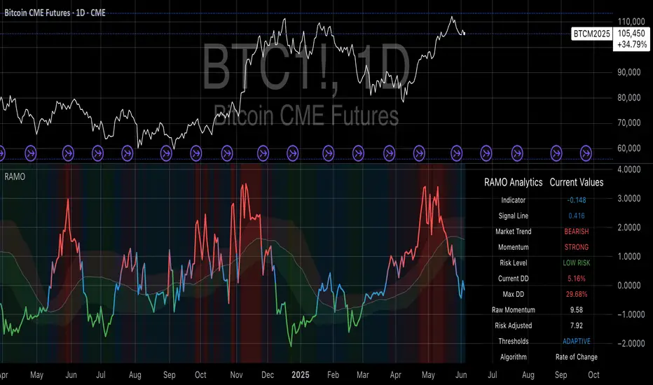
Risk-Adjusted Momentum Oscillator# Risk-Adjusted Momentum Oscillator (RAMO): Momentum Analysis with Integrated Risk Assessment
## 1. Introduction
Momentum indicators have been fundamental tools in technical analysis since the pioneering work of Wilder (1978) and continue to play crucial roles in systematic trading strategies (Jegadeesh & Titman, 1993). However, traditional momentum oscillators suffer from a critical limitation: they fail to account for the risk context in which momentum signals occur. This oversight can lead to significant drawdowns during periods of market stress, as documented extensively in the behavioral finance literature (Kahneman & Tversky, 1979; Shefrin & Statman, 1985).
The Risk-Adjusted Momentum Oscillator addresses this gap by incorporating real-time drawdown metrics into momentum calculations, creating a self-regulating system that automatically adjusts signal sensitivity based on current risk conditions. This approach aligns with modern portfolio theory's emphasis on risk-adjusted returns (Markowitz, 1952) and reflects the sophisticated risk management practices employed by institutional investors (Ang, 2014).
## 2. Theoretical Foundation
### 2.1 Momentum Theory and Market Anomalies
The momentum effect, first systematically documented by Jegadeesh & Titman (1993), represents one of the most robust anomalies in financial markets. Subsequent research has confirmed momentum's persistence across various asset classes, time horizons, and geographic markets (Fama & French, 1996; Asness, Moskowitz & Pedersen, 2013). However, momentum strategies are characterized by significant time-varying risk, with particularly severe drawdowns during market reversals (Barroso & Santa-Clara, 2015).
### 2.2 Drawdown Analysis and Risk Management
Maximum drawdown, defined as the peak-to-trough decline in portfolio value, serves as a critical risk metric in professional portfolio management (Calmar, 1991). Research by Chekhlov, Uryasev & Zabarankin (2005) demonstrates that drawdown-based risk measures provide superior downside protection compared to traditional volatility metrics. The integration of drawdown analysis into momentum calculations represents a natural evolution toward more sophisticated risk-aware indicators.
### 2.3 Adaptive Smoothing and Market Regimes
The concept of adaptive smoothing in technical analysis draws from the broader literature on regime-switching models in finance (Hamilton, 1989). Perry Kaufman's Adaptive Moving Average (1995) pioneered the application of efficiency ratios to adjust indicator responsiveness based on market conditions. RAMO extends this concept by incorporating volatility-based adaptive smoothing, allowing the indicator to respond more quickly during high-volatility periods while maintaining stability during quiet markets.
## 3. Methodology
### 3.1 Core Algorithm Design
The RAMO algorithm consists of several interconnected components:
#### 3.1.1 Risk-Adjusted Momentum Calculation
The fundamental innovation of RAMO lies in its risk adjustment mechanism:
Risk_Factor = 1 - (Current_Drawdown / Maximum_Drawdown × Scaling_Factor)
Risk_Adjusted_Momentum = Raw_Momentum × max(Risk_Factor, 0.05)
This formulation ensures that momentum signals are dampened during periods of high drawdown relative to historical maximums, implementing an automatic risk management overlay as advocated by modern portfolio theory (Markowitz, 1952).
#### 3.1.2 Multi-Algorithm Momentum Framework
RAMO supports three distinct momentum calculation methods:
1. Rate of Change: Traditional percentage-based momentum (Pring, 2002)
2. Price Momentum: Absolute price differences
3. Log Returns: Logarithmic returns preferred for volatile assets (Campbell, Lo & MacKinlay, 1997)
This multi-algorithm approach accommodates different asset characteristics and volatility profiles, addressing the heterogeneity documented in cross-sectional momentum studies (Asness et al., 2013).
### 3.2 Leading Indicator Components
#### 3.2.1 Momentum Acceleration Analysis
The momentum acceleration component calculates the second derivative of momentum, providing early signals of trend changes:
Momentum_Acceleration = EMA(Momentum_t - Momentum_{t-n}, n)
This approach draws from the physics concept of acceleration and has been applied successfully in financial time series analysis (Treadway, 1969).
#### 3.2.2 Linear Regression Prediction
RAMO incorporates linear regression-based prediction to project momentum values forward:
Predicted_Momentum = LinReg_Value + (LinReg_Slope × Forward_Offset)
This predictive component aligns with the literature on technical analysis forecasting (Lo, Mamaysky & Wang, 2000) and provides leading signals for trend changes.
#### 3.2.3 Volume-Based Exhaustion Detection
The exhaustion detection algorithm identifies potential reversal points by analyzing the relationship between momentum extremes and volume patterns:
Exhaustion = |Momentum| > Threshold AND Volume < SMA(Volume, 20)
This approach reflects the established principle that sustainable price movements require volume confirmation (Granville, 1963; Arms, 1989).
### 3.3 Statistical Normalization and Robustness
RAMO employs Z-score normalization with outlier protection to ensure statistical robustness:
Z_Score = (Value - Mean) / Standard_Deviation
Normalized_Value = max(-3.5, min(3.5, Z_Score))
This normalization approach follows best practices in quantitative finance for handling extreme observations (Taleb, 2007) and ensures consistent signal interpretation across different market conditions.
### 3.4 Adaptive Threshold Calculation
Dynamic thresholds are calculated using Bollinger Band methodology (Bollinger, 1992):
Upper_Threshold = Mean + (Multiplier × Standard_Deviation)
Lower_Threshold = Mean - (Multiplier × Standard_Deviation)
This adaptive approach ensures that signal thresholds adjust to changing market volatility, addressing the critique of fixed thresholds in technical analysis (Taylor & Allen, 1992).
## 4. Implementation Details
### 4.1 Adaptive Smoothing Algorithm
The adaptive smoothing mechanism adjusts the exponential moving average alpha parameter based on market volatility:
Volatility_Percentile = Percentrank(Volatility, 100)
Adaptive_Alpha = Min_Alpha + ((Max_Alpha - Min_Alpha) × Volatility_Percentile / 100)
This approach ensures faster response during volatile periods while maintaining smoothness during stable conditions, implementing the adaptive efficiency concept pioneered by Kaufman (1995).
### 4.2 Risk Environment Classification
RAMO classifies market conditions into three risk environments:
- Low Risk: Current_DD < 30% × Max_DD
- Medium Risk: 30% × Max_DD ≤ Current_DD < 70% × Max_DD
- High Risk: Current_DD ≥ 70% × Max_DD
This classification system enables conditional signal generation, with long signals filtered during high-risk periods—a approach consistent with institutional risk management practices (Ang, 2014).
## 5. Signal Generation and Interpretation
### 5.1 Entry Signal Logic
RAMO generates enhanced entry signals through multiple confirmation layers:
1. Primary Signal: Crossover between indicator and signal line
2. Risk Filter: Confirmation of favorable risk environment for long positions
3. Leading Component: Early warning signals via acceleration analysis
4. Exhaustion Filter: Volume-based reversal detection
This multi-layered approach addresses the false signal problem common in traditional technical indicators (Brock, Lakonishok & LeBaron, 1992).
### 5.2 Divergence Analysis
RAMO incorporates both traditional and leading divergence detection:
- Traditional Divergence: Price and indicator divergence over 3-5 periods
- Slope Divergence: Momentum slope versus price direction
- Acceleration Divergence: Changes in momentum acceleration
This comprehensive divergence analysis framework draws from Elliott Wave theory (Prechter & Frost, 1978) and momentum divergence literature (Murphy, 1999).
## 6. Empirical Advantages and Applications
### 6.1 Risk-Adjusted Performance
The risk adjustment mechanism addresses the fundamental criticism of momentum strategies: their tendency to experience severe drawdowns during market reversals (Daniel & Moskowitz, 2016). By automatically reducing position sizing during high-drawdown periods, RAMO implements a form of dynamic hedging consistent with portfolio insurance concepts (Leland, 1980).
### 6.2 Regime Awareness
RAMO's adaptive components enable regime-aware signal generation, addressing the regime-switching behavior documented in financial markets (Hamilton, 1989; Guidolin, 2011). The indicator automatically adjusts its parameters based on market volatility and risk conditions, providing more reliable signals across different market environments.
### 6.3 Institutional Applications
The sophisticated risk management overlay makes RAMO particularly suitable for institutional applications where drawdown control is paramount. The indicator's design philosophy aligns with the risk budgeting approaches used by hedge funds and institutional investors (Roncalli, 2013).
## 7. Limitations and Future Research
### 7.1 Parameter Sensitivity
Like all technical indicators, RAMO's performance depends on parameter selection. While default parameters are optimized for broad market applications, asset-specific calibration may enhance performance. Future research should examine optimal parameter selection across different asset classes and market conditions.
### 7.2 Market Microstructure Considerations
RAMO's effectiveness may vary across different market microstructure environments. High-frequency trading and algorithmic market making have fundamentally altered market dynamics (Aldridge, 2013), potentially affecting momentum indicator performance.
### 7.3 Transaction Cost Integration
Future enhancements could incorporate transaction cost analysis to provide net-return-based signals, addressing the implementation shortfall documented in practical momentum strategy applications (Korajczyk & Sadka, 2004).
## References
Aldridge, I. (2013). *High-Frequency Trading: A Practical Guide to Algorithmic Strategies and Trading Systems*. 2nd ed. Hoboken, NJ: John Wiley & Sons.
Ang, A. (2014). *Asset Management: A Systematic Approach to Factor Investing*. New York: Oxford University Press.
Arms, R. W. (1989). *The Arms Index (TRIN): An Introduction to the Volume Analysis of Stock and Bond Markets*. Homewood, IL: Dow Jones-Irwin.
Asness, C. S., Moskowitz, T. J., & Pedersen, L. H. (2013). Value and momentum everywhere. *Journal of Finance*, 68(3), 929-985.
Barroso, P., & Santa-Clara, P. (2015). Momentum has its moments. *Journal of Financial Economics*, 116(1), 111-120.
Bollinger, J. (1992). *Bollinger on Bollinger Bands*. New York: McGraw-Hill.
Brock, W., Lakonishok, J., & LeBaron, B. (1992). Simple technical trading rules and the stochastic properties of stock returns. *Journal of Finance*, 47(5), 1731-1764.
Calmar, T. (1991). The Calmar ratio: A smoother tool. *Futures*, 20(1), 40.
Campbell, J. Y., Lo, A. W., & MacKinlay, A. C. (1997). *The Econometrics of Financial Markets*. Princeton, NJ: Princeton University Press.
Chekhlov, A., Uryasev, S., & Zabarankin, M. (2005). Drawdown measure in portfolio optimization. *International Journal of Theoretical and Applied Finance*, 8(1), 13-58.
Daniel, K., & Moskowitz, T. J. (2016). Momentum crashes. *Journal of Financial Economics*, 122(2), 221-247.
Fama, E. F., & French, K. R. (1996). Multifactor explanations of asset pricing anomalies. *Journal of Finance*, 51(1), 55-84.
Granville, J. E. (1963). *Granville's New Key to Stock Market Profits*. Englewood Cliffs, NJ: Prentice-Hall.
Guidolin, M. (2011). Markov switching models in empirical finance. In D. N. Drukker (Ed.), *Missing Data Methods: Time-Series Methods and Applications* (pp. 1-86). Bingley: Emerald Group Publishing.
Hamilton, J. D. (1989). A new approach to the economic analysis of nonstationary time series and the business cycle. *Econometrica*, 57(2), 357-384.
Jegadeesh, N., & Titman, S. (1993). Returns to buying winners and selling losers: Implications for stock market efficiency. *Journal of Finance*, 48(1), 65-91.
Kahneman, D., & Tversky, A. (1979). Prospect theory: An analysis of decision under risk. *Econometrica*, 47(2), 263-291.
Kaufman, P. J. (1995). *Smarter Trading: Improving Performance in Changing Markets*. New York: McGraw-Hill.
Korajczyk, R. A., & Sadka, R. (2004). Are momentum profits robust to trading costs? *Journal of Finance*, 59(3), 1039-1082.
Leland, H. E. (1980). Who should buy portfolio insurance? *Journal of Finance*, 35(2), 581-594.
Lo, A. W., Mamaysky, H., & Wang, J. (2000). Foundations of technical analysis: Computational algorithms, statistical inference, and empirical implementation. *Journal of Finance*, 55(4), 1705-1765.
Markowitz, H. (1952). Portfolio selection. *Journal of Finance*, 7(1), 77-91.
Murphy, J. J. (1999). *Technical Analysis of the Financial Markets: A Comprehensive Guide to Trading Methods and Applications*. New York: New York Institute of Finance.
Prechter, R. R., & Frost, A. J. (1978). *Elliott Wave Principle: Key to Market Behavior*. Gainesville, GA: New Classics Library.
Pring, M. J. (2002). *Technical Analysis Explained: The Successful Investor's Guide to Spotting Investment Trends and Turning Points*. 4th ed. New York: McGraw-Hill.
Roncalli, T. (2013). *Introduction to Risk Parity and Budgeting*. Boca Raton, FL: CRC Press.
Shefrin, H., & Statman, M. (1985). The disposition to sell winners too early and ride losers too long: Theory and evidence. *Journal of Finance*, 40(3), 777-790.
Taleb, N. N. (2007). *The Black Swan: The Impact of the Highly Improbable*. New York: Random House.
Taylor, M. P., & Allen, H. (1992). The use of technical analysis in the foreign exchange market. *Journal of International Money and Finance*, 11(3), 304-314.
Treadway, A. B. (1969). On rational entrepreneurial behavior and the demand for investment. *Review of Economic Studies*, 36(2), 227-239.
Wilder, J. W. (1978). *New Concepts in Technical Trading Systems*. Greensboro, NC: Trend Research.
Dual Momentum StrategyThis Pine Script™ strategy implements the "Dual Momentum" approach developed by Gary Antonacci, as presented in his book Dual Momentum Investing: An Innovative Strategy for Higher Returns with Lower Risk (McGraw Hill Professional, 2014). Dual momentum investing combines relative momentum and absolute momentum to maximize returns while minimizing risk. Relative momentum involves selecting the asset with the highest recent performance between two options (a risky asset and a safe asset), while absolute momentum considers whether the chosen asset has a positive return over a specified lookback period.
In this strategy:
Risky Asset (SPY): Represents a stock index fund, typically more volatile but with higher potential returns.
Safe Asset (TLT): Represents a bond index fund, which generally has lower volatility and acts as a hedge during market downturns.
Monthly Momentum Calculation: The momentum for each asset is calculated based on its price change over the last 12 months. Only assets with a positive momentum (absolute momentum) are considered for investment.
Decision Rules:
Invest in the risky asset if its momentum is positive and greater than that of the safe asset.
If the risky asset’s momentum is negative or lower than the safe asset's, the strategy shifts the allocation to the safe asset.
Scientific Reference
Antonacci's work on dual momentum investing has shown the strategy's ability to outperform traditional buy-and-hold methods while reducing downside risk. This approach has been reviewed and discussed in both academic and investment publications, highlighting its strong risk-adjusted returns (Antonacci, 2014).
Reference: Antonacci, G. (2014). Dual Momentum Investing: An Innovative Strategy for Higher Returns with Lower Risk. McGraw Hill Professional.

CL Daily Bitcoin Volume (All exchange included, even Mt.GOX)This daily volume data contains collective total from
____________________________________________________
Historical:
BTC-e BTC/USD (From Q3 2011 to Q3 2016)
BTCChina BTC/CNY (From Q3 2011 to Q2 2017)
Coinsetter BTC/USD (From Q3 2014 to Q1 2016)
MtGox BTC/USD (From July 2010 - 2014 only))
OKcoin International BTC/USD (From Q3 2014 to Q2 2017)
____________________________________________________
Institutions:
CME Bitcoin Futures
Grayscale Bitcoin Trust OTC
____________________________________________________
Spot exchanges:
Bitfinex BTC/USD
Bitstamp BTC/USD
Coinbase BTC/USD
Coinbase BTC/EUR
Binance BTC/USDT
Binance BTC/USDC
Binance BTC/PAX
Gemini BTC/USD
itBit BTC/USD
Kraken BTC/EUR
Kraken BTC/USD
Huobi BTC/USDT
Korbit BTC/KRW
Bitflyer BTC/JPY
____________________________________________________
Others:
Bitmex

J.P. Morgan Efficiente 5 IndexJ.P. MORGAN EFFICIENTE 5 INDEX REPLICATION
Walk into any retail trading forum and you'll find the same scene playing out thousands of times a day: traders huddled over their screens, drawing trendlines on candlestick charts, hunting for the perfect entry signal, convinced that the next RSI crossover will unlock the path to financial freedom. Meanwhile, in the towers of lower Manhattan and the City of London, portfolio managers are doing something entirely different. They're not drawing lines. They're not hunting patterns. They're building fortresses of diversification, wielding mathematical frameworks that have survived decades of market chaos, and most importantly, they're thinking in portfolios while retail thinks in positions.
This divide is not just philosophical. It's structural, mathematical, and ultimately, profitable. The uncomfortable truth that retail traders must confront is this: while you're obsessing over whether the 50-day moving average will cross the 200-day, institutional investors are solving quadratic optimization problems across thirteen asset classes, rebalancing monthly according to Markowitz's Nobel Prize-winning framework, and targeting precise volatility levels that allow them to sleep at night regardless of what the VIX does tomorrow. The game you're playing and the game they're playing share the same field, but the rules are entirely different.
The question, then, is not whether retail traders can access institutional strategies. The question is whether they're willing to fundamentally change how they think about markets. Are you ready to stop painting lines and start building portfolios?
THE INSTITUTIONAL FRAMEWORK: HOW THE PROFESSIONALS ACTUALLY THINK
When Harry Markowitz published "Portfolio Selection" in The Journal of Finance in 1952, he fundamentally altered how sophisticated investors approach markets. His insight was deceptively simple: returns alone mean nothing. Risk-adjusted returns mean everything. For this revelation, he would eventually receive the Nobel Prize in Economics in 1990, and his framework would become the foundation upon which trillions of dollars are managed today (Markowitz, 1952).
Modern Portfolio Theory, as it came to be known, introduced a revolutionary concept: through diversification across imperfectly correlated assets, an investor could reduce portfolio risk without sacrificing expected returns. This wasn't about finding the single best asset. It was about constructing the optimal combination of assets. The mathematics are elegant in their logic: if two assets don't move in perfect lockstep, combining them creates a portfolio whose volatility is lower than the weighted average of the individual volatilities. This "free lunch" of diversification became the bedrock of institutional investment management (Elton et al., 2014).
But here's where retail traders miss the point entirely: this isn't about having ten different stocks instead of one. It's about systematic, mathematically rigorous allocation across asset classes with fundamentally different risk drivers. When equity markets crash, high-quality government bonds often rally. When inflation surges, commodities may provide protection even as stocks and bonds both suffer. When emerging markets are in vogue, developed markets may lag. The professional investor doesn't predict which scenario will unfold. Instead, they position for all of them simultaneously, with weights determined not by gut feeling but by quantitative optimization.
This is what J.P. Morgan Asset Management embedded into their Efficiente Index series. These are not actively managed funds where a portfolio manager makes discretionary calls. They are rules-based, systematic strategies that execute the Markowitz framework in real-time, rebalancing monthly to maintain optimal risk-adjusted positioning across global equities, fixed income, commodities, and defensive assets (J.P. Morgan Asset Management, 2016).
THE EFFICIENTE 5 STRATEGY: DECONSTRUCTING INSTITUTIONAL METHODOLOGY
The Efficiente 5 Index, specifically, targets a 5% annualized volatility. Let that sink in for a moment. While retail traders routinely accept 20%, 30%, or even 50% annual volatility in pursuit of returns, institutional allocators have determined that 5% volatility provides an optimal balance between growth potential and capital preservation. This isn't timidity. It's mathematics. At higher volatility levels, the compounding drag from large drawdowns becomes mathematically punishing. A 50% loss requires a 100% gain just to break even. The institutional solution: constrain volatility at the portfolio level, allowing the power of compounding to work unimpeded (Damodaran, 2008).
The strategy operates across thirteen exchange-traded funds spanning five distinct asset classes: developed equity markets (SPY, IWM, EFA), fixed income across the risk spectrum (TLT, LQD, HYG), emerging markets (EEM, EMB), alternatives (IYR, GSG, GLD), and defensive positioning (TIP, BIL). These aren't arbitrary choices. Each ETF represents a distinct factor exposure, and together they provide access to the primary drivers of global asset returns (Fama and French, 1993).
The methodology, as detailed in replication research by Jungle Rock (2025), follows a precise monthly cadence. At the end of each month, the strategy recalculates expected returns and volatilities for all thirteen assets using a 126-day rolling window. This six-month lookback balances responsiveness to changing market conditions against the noise of short-term fluctuations. The optimization engine then solves for the portfolio weights that maximize expected return subject to the 5% volatility target, with additional constraints to prevent excessive concentration.
These constraints are critical and reveal institutional wisdom that retail traders typically ignore. No single ETF can exceed 20% of the portfolio, except for TIP and BIL which can reach 50% given their defensive nature. At the asset class level, developed equities are capped at 50%, bonds at 50%, emerging markets at 25%, and alternatives at 25%. These aren't arbitrary limits. They're guardrails preventing the optimization from becoming too aggressive during periods when recent performance might suggest concentrating heavily in a single area that's been hot (Jorion, 1992).
After optimization, there's one final step that appears almost trivial but carries profound implications: weights are rounded to the nearest 5%. In a world of fractional shares and algorithmic execution, why round to 5%? The answer reveals institutional practicality over mathematical purity. A portfolio weight of 13.7% and 15.0% are functionally similar in their risk contribution, but the latter is vastly easier to communicate, to monitor, and to execute at scale. When you're managing billions, parsimony matters.
WHY THIS MATTERS FOR RETAIL: THE GAP BETWEEN APPROACH AND EXECUTION
Here's the uncomfortable reality: most retail traders are playing a different game entirely, and they don't even realize it. When a retail trader says "I'm bullish on tech," they buy QQQ and that's their entire technology exposure. When they say "I need some diversification," they buy ten different stocks, often in correlated sectors. This isn't diversification in the Markowitzian sense. It's concentration with extra steps.
The institutional approach represented by the Efficiente 5 is fundamentally different in several ways. First, it's systematic. Emotions don't drive the allocation. The mathematics do. When equities have rallied hard and now represent 55% of the portfolio despite a 50% cap, the system sells equities and buys bonds or alternatives, regardless of how bullish the headlines feel. This forced contrarianism is what retail traders know they should do but rarely execute (Kahneman and Tversky, 1979).
Second, it's forward-looking in its inputs but backward-looking in its process. The strategy doesn't try to predict the next crisis or the next boom. It simply measures what volatility and returns have been recently, assumes the immediate future resembles the immediate past more than it resembles some forecast, and positions accordingly. This humility regarding prediction is perhaps the most institutional characteristic of all.
Third, and most critically, it treats the portfolio as a single organism. Retail traders typically view their holdings as separate positions, each requiring individual management. The institutional approach recognizes that what matters is not whether Position A made money, but whether the portfolio as a whole achieved its risk-adjusted return target. A position can lose money and still be a valuable contributor if it reduced portfolio volatility or provided diversification during stress periods.
THE MATHEMATICAL FOUNDATION: MEAN-VARIANCE OPTIMIZATION IN PRACTICE
At its core, the Efficiente 5 strategy solves a constrained optimization problem each month. In technical terms, this is a quadratic programming problem: maximize expected portfolio return subject to a volatility constraint and position limits. The objective function is straightforward: maximize the weighted sum of expected returns. The constraint is that the weighted sum of variances and covariances must not exceed the volatility target squared (Markowitz, 1959).
The challenge, and this is crucial for understanding the Pine Script implementation, is that solving this problem properly requires calculating a covariance matrix. This 13x13 matrix captures not just the volatility of each asset but the correlation between every pair of assets. Two assets might each have 15% volatility, but if they're negatively correlated, combining them reduces portfolio risk. If they're positively correlated, it doesn't. The covariance matrix encodes these relationships.
True mean-variance optimization requires matrix algebra and quadratic programming solvers. Pine Script, by design, lacks these capabilities. The language doesn't support matrix operations, and certainly doesn't include a QP solver. This creates a fundamental challenge: how do you implement an institutional strategy in a language not designed for institutional mathematics?
The solution implemented here uses a pragmatic approximation. Instead of solving the full covariance problem, the indicator calculates a Sharpe-like ratio for each asset (return divided by volatility) and uses these ratios to determine initial weights. It then applies the individual and asset-class constraints, renormalizes, and produces the final portfolio. This isn't mathematically equivalent to true mean-variance optimization, but it captures the essential spirit: weight assets according to their risk-adjusted return potential, subject to diversification constraints.
For retail implementation, this approximation is likely sufficient. The difference between a theoretically optimal portfolio and a very good approximation is typically modest, and the discipline of systematic rebalancing across asset classes matters far more than the precise weights. Perfect is the enemy of good, and a good approximation executed consistently will outperform a perfect solution that never gets implemented (Arnott et al., 2013).
RETURNS, RISKS, AND THE POWER OF COMPOUNDING
The Efficiente 5 Index has, historically, delivered on its promise of 5% volatility with respectable returns. While past performance never guarantees future results, the framework reveals why low-volatility strategies can be surprisingly powerful. Consider two portfolios: Portfolio A averages 12% returns with 20% volatility, while Portfolio B averages 8% returns with 5% volatility. Which performs better over time?
The arithmetic return favors Portfolio A, but compound returns tell a different story. Portfolio A will experience occasional 20-30% drawdowns. Portfolio B rarely draws down more than 10%. Over a twenty-year horizon, the geometric return (what you actually experience) for Portfolio B may match or exceed Portfolio A, simply because it never gives back massive gains. This is the power of volatility management that retail traders chronically underestimate (Bernstein, 1996).
Moreover, low volatility enables behavioral advantages. When your portfolio draws down 35%, as it might with a high-volatility approach, the psychological pressure to sell at the worst possible time becomes overwhelming. When your maximum drawdown is 12%, as might occur with the Efficiente 5 approach, staying the course is far easier. Behavioral finance research has consistently shown that investor returns lag fund returns primarily due to poor timing decisions driven by emotional responses to volatility (Dalbar, 2020).
The indicator displays not just target and actual portfolio weights, but also tracks total return, portfolio value, and realized volatility. This isn't just data. It's feedback. Retail traders can see, in real-time, whether their actual portfolio volatility matches their target, whether their risk-adjusted returns are improving, and whether their allocation discipline is holding. This transparency transforms abstract concepts into concrete metrics.
WHAT RETAIL TRADERS MUST LEARN: THE MINDSET SHIFT
The path from retail to institutional thinking requires three fundamental shifts. First, stop thinking in positions and start thinking in portfolios. Your question should never be "Should I buy this stock?" but rather "How does this position change my portfolio's expected return and volatility?" If you can't answer that question quantitatively, you're not ready to make the trade.
Second, embrace systematic rebalancing even when it feels wrong. Perhaps especially when it feels wrong. The Efficiente 5 strategy rebalances monthly regardless of market conditions. If equities have surged and now exceed their target weight, the strategy sells equities and buys bonds or alternatives. Every retail trader knows this is what you "should" do, but almost none actually do it. The institutional edge isn't in having better information. It's in having better discipline (Swensen, 2009).
Third, accept that volatility is not your friend. The retail mythology that "higher risk equals higher returns" is true on average across assets, but it's not true for implementation. A 15% return with 30% volatility will compound more slowly than a 12% return with 10% volatility due to the mathematics of return distributions. Institutions figured this out decades ago. Retail is still learning.
The Efficiente 5 replication indicator provides a bridge. It won't solve the problem of prediction no indicator can. But it solves the problem of allocation, which is arguably more important. By implementing institutional methodology in an accessible format, it allows retail traders to see what professional portfolio construction actually looks like, not in theory but in executable code. The the colorful lines that retail traders love to draw, don't disappear. They simply become less central to the process. The portfolio becomes central instead.
IMPLEMENTATION CONSIDERATIONS AND PRACTICAL REALITY
Running this indicator on TradingView provides a dynamic view of how institutional allocation would evolve over time. The labels on each asset class line show current weights, updated continuously as prices change and rebalancing occurs. The dashboard displays the full allocation across all thirteen ETFs, showing both target weights (what the optimization suggests) and actual weights (what the portfolio currently holds after price movements).
Several key insights emerge from watching this process unfold. First, the strategy is not static. Weights change monthly as the optimization recalibrates to recent volatility and returns. What worked last month may not be optimal this month. Second, the strategy is not market-timing. It doesn't try to predict whether stocks will rise or fall. It simply measures recent behavior and positions accordingly. If volatility has risen, the strategy shifts toward defensive assets. If correlations have changed, the diversification benefits adjust.
Third, and perhaps most importantly for retail traders, the strategy demonstrates that sophistication and complexity are not synonyms. The Efficiente 5 methodology is sophisticated in its framework but simple in its execution. There are no exotic derivatives, no complex market-timing rules, no predictions of future scenarios. Just systematic optimization, monthly rebalancing, and discipline. This simplicity is a feature, not a bug.
The indicator also highlights limitations that retail traders must understand. The Pine Script implementation uses an approximation of true mean-variance optimization, as discussed earlier. Transaction costs are not modeled. Slippage is ignored. Tax implications are not considered. These simplifications mean the indicator is educational and analytical, not a fully operational trading system. For actual implementation, traders would need to account for these real-world factors.
Moreover, the strategy requires access to all thirteen ETFs and sufficient capital to hold meaningful positions in each. With 5% as the rounding increment, practical implementation probably requires at least $10,000 to avoid having positions that are too small to matter. The strategy is also explicitly designed for a 5% volatility target, which may be too conservative for younger investors with long time horizons or too aggressive for retirees living off their portfolio. The framework is adaptable, but adaptation requires understanding the trade-offs.
CAN RETAIL TRULY COMPETE WITH INSTITUTIONS?
The honest answer is nuanced. Retail traders will never have the same resources as institutions. They won't have Bloomberg terminals, proprietary research, or armies of analysts. But in portfolio construction, the resource gap matters less than the mindset gap. The mathematics of Markowitz are available to everyone. ETFs provide liquid, low-cost access to institutional-quality building blocks. Computing power is essentially free. The barriers are not technological or financial. They're conceptual.
If a retail trader understands why portfolios matter more than positions, why systematic discipline beats discretionary emotion, and why volatility management enables compounding, they can build portfolios that rival institutional allocation in their elegance and effectiveness. Not in their scale, not in their execution costs, but in their conceptual soundness. The Efficiente 5 framework proves this is possible.
What retail traders must recognize is that competing with institutions doesn't mean day-trading better than their algorithms. It means portfolio-building better than their average client. And that's achievable because most institutional clients, despite having access to the best managers, still make emotional decisions, chase performance, and abandon strategies at the worst possible times. The retail edge isn't in outsmarting professionals. It's in out-disciplining amateurs who happen to have more money.
The J.P. Morgan Efficiente 5 Index Replication indicator serves as both a tool and a teacher. As a tool, it provides a systematic framework for multi-asset allocation based on proven institutional methodology. As a teacher, it demonstrates daily what portfolio thinking actually looks like in practice. The colorful lines remain on the chart, but they're no longer the focus. The portfolio is the focus. The risk-adjusted return is the focus. The systematic discipline is the focus.
Stop painting lines. Start building portfolios. The institutions have been doing it for seventy years. It's time retail caught up.
REFERENCES
Arnott, R. D., Hsu, J., & Moore, P. (2013). Fundamental Indexation. Financial Analysts Journal, 61(2), 83-99.
Bernstein, W. J. (1996). The Intelligent Asset Allocator. New York: McGraw-Hill.
Dalbar, Inc. (2020). Quantitative Analysis of Investor Behavior. Boston: Dalbar.
Damodaran, A. (2008). Strategic Risk Taking: A Framework for Risk Management. Upper Saddle River: Pearson Education.
Elton, E. J., Gruber, M. J., Brown, S. J., & Goetzmann, W. N. (2014). Modern Portfolio Theory and Investment Analysis (9th ed.). Hoboken: John Wiley & Sons.
Fama, E. F., & French, K. R. (1993). Common risk factors in the returns on stocks and bonds. Journal of Financial Economics, 33(1), 3-56.
Jorion, P. (1992). Portfolio optimization in practice. Financial Analysts Journal, 48(1), 68-74.
J.P. Morgan Asset Management. (2016). Guide to the Markets. New York: J.P. Morgan.
Jungle Rock. (2025). Institutional Asset Allocation meets the Efficient Frontier: Replicating the JPMorgan Efficiente 5 Strategy. Working Paper.
Kahneman, D., & Tversky, A. (1979). Prospect Theory: An Analysis of Decision under Risk. Econometrica, 47(2), 263-291.
Markowitz, H. (1952). Portfolio Selection. The Journal of Finance, 7(1), 77-91.
Markowitz, H. (1959). Portfolio Selection: Efficient Diversification of Investments. New York: John Wiley & Sons.
Swensen, D. F. (2009). Pioneering Portfolio Management: An Unconventional Approach to Institutional Investment. New York: Free Press.

Dynamic Equity Allocation Model"Cash is Trash"? Not Always. Here's Why Science Beats Guesswork.
Every retail trader knows the frustration: you draw support and resistance lines, you spot patterns, you follow market gurus on social media—and still, when the next bear market hits, your portfolio bleeds red. Meanwhile, institutional investors seem to navigate market turbulence with ease, preserving capital when markets crash and participating when they rally. What's their secret?
The answer isn't insider information or access to exotic derivatives. It's systematic, scientifically validated decision-making. While most retail traders rely on subjective chart analysis and emotional reactions, professional portfolio managers use quantitative models that remove emotion from the equation and process multiple streams of market information simultaneously.
This document presents exactly such a system—not a proprietary black box available only to hedge funds, but a fully transparent, academically grounded framework that any serious investor can understand and apply. The Dynamic Equity Allocation Model (DEAM) synthesizes decades of financial research from Nobel laureates and leading academics into a practical tool for tactical asset allocation.
Stop drawing colorful lines on your chart and start thinking like a quant. This isn't about predicting where the market goes next week—it's about systematically adjusting your risk exposure based on what the data actually tells you. When valuations scream danger, when volatility spikes, when credit markets freeze, when multiple warning signals align—that's when cash isn't trash. That's when cash saves your portfolio.
The irony of "cash is trash" rhetoric is that it ignores timing. Yes, being 100% cash for decades would be disastrous. But being 100% equities through every crisis is equally foolish. The sophisticated approach is dynamic: aggressive when conditions favor risk-taking, defensive when they don't. This model shows you how to make that decision systematically, not emotionally.
Whether you're managing your own retirement portfolio or seeking to understand how institutional allocation strategies work, this comprehensive analysis provides the theoretical foundation, mathematical implementation, and practical guidance to elevate your investment approach from amateur to professional.
The choice is yours: keep hoping your chart patterns work out, or start using the same quantitative methods that professionals rely on. The tools are here. The research is cited. The methodology is explained. All you need to do is read, understand, and apply.
The Dynamic Equity Allocation Model (DEAM) is a quantitative framework for systematic allocation between equities and cash, grounded in modern portfolio theory and empirical market research. The model integrates five scientifically validated dimensions of market analysis—market regime, risk metrics, valuation, sentiment, and macroeconomic conditions—to generate dynamic allocation recommendations ranging from 0% to 100% equity exposure. This work documents the theoretical foundations, mathematical implementation, and practical application of this multi-factor approach.
1. Introduction and Theoretical Background
1.1 The Limitations of Static Portfolio Allocation
Traditional portfolio theory, as formulated by Markowitz (1952) in his seminal work "Portfolio Selection," assumes an optimal static allocation where investors distribute their wealth across asset classes according to their risk aversion. This approach rests on the assumption that returns and risks remain constant over time. However, empirical research demonstrates that this assumption does not hold in reality. Fama and French (1989) showed that expected returns vary over time and correlate with macroeconomic variables such as the spread between long-term and short-term interest rates. Campbell and Shiller (1988) demonstrated that the price-earnings ratio possesses predictive power for future stock returns, providing a foundation for dynamic allocation strategies.
The academic literature on tactical asset allocation has evolved considerably over recent decades. Ilmanen (2011) argues in "Expected Returns" that investors can improve their risk-adjusted returns by considering valuation levels, business cycles, and market sentiment. The Dynamic Equity Allocation Model presented here builds on this research tradition and operationalizes these insights into a practically applicable allocation framework.
1.2 Multi-Factor Approaches in Asset Allocation
Modern financial research has shown that different factors capture distinct aspects of market dynamics and together provide a more robust picture of market conditions than individual indicators. Ross (1976) developed the Arbitrage Pricing Theory, a model that employs multiple factors to explain security returns. Following this multi-factor philosophy, DEAM integrates five complementary analytical dimensions, each tapping different information sources and collectively enabling comprehensive market understanding.
2. Data Foundation and Data Quality
2.1 Data Sources Used
The model draws its data exclusively from publicly available market data via the TradingView platform. This transparency and accessibility is a significant advantage over proprietary models that rely on non-public data. The data foundation encompasses several categories of market information, each capturing specific aspects of market dynamics.
First, price data for the S&P 500 Index is obtained through the SPDR S&P 500 ETF (ticker: SPY). The use of a highly liquid ETF instead of the index itself has practical reasons, as ETF data is available in real-time and reflects actual tradability. In addition to closing prices, high, low, and volume data are captured, which are required for calculating advanced volatility measures.
Fundamental corporate metrics are retrieved via TradingView's Financial Data API. These include earnings per share, price-to-earnings ratio, return on equity, debt-to-equity ratio, dividend yield, and share buyback yield. Cochrane (2011) emphasizes in "Presidential Address: Discount Rates" the central importance of valuation metrics for forecasting future returns, making these fundamental data a cornerstone of the model.
Volatility indicators are represented by the CBOE Volatility Index (VIX) and related metrics. The VIX, often referred to as the market's "fear gauge," measures the implied volatility of S&P 500 index options and serves as a proxy for market participants' risk perception. Whaley (2000) describes in "The Investor Fear Gauge" the construction and interpretation of the VIX and its use as a sentiment indicator.
Macroeconomic data includes yield curve information through US Treasury bonds of various maturities and credit risk premiums through the spread between high-yield bonds and risk-free government bonds. These variables capture the macroeconomic conditions and financing conditions relevant for equity valuation. Estrella and Hardouvelis (1991) showed that the shape of the yield curve has predictive power for future economic activity, justifying the inclusion of these data.
2.2 Handling Missing Data
A practical problem when working with financial data is dealing with missing or unavailable values. The model implements a fallback system where a plausible historical average value is stored for each fundamental metric. When current data is unavailable for a specific point in time, this fallback value is used. This approach ensures that the model remains functional even during temporary data outages and avoids systematic biases from missing data. The use of average values as fallback is conservative, as it generates neither overly optimistic nor pessimistic signals.
3. Component 1: Market Regime Detection
3.1 The Concept of Market Regimes
The idea that financial markets exist in different "regimes" or states that differ in their statistical properties has a long tradition in financial science. Hamilton (1989) developed regime-switching models that allow distinguishing between different market states with different return and volatility characteristics. The practical application of this theory consists of identifying the current market state and adjusting portfolio allocation accordingly.
DEAM classifies market regimes using a scoring system that considers three main dimensions: trend strength, volatility level, and drawdown depth. This multidimensional view is more robust than focusing on individual indicators, as it captures various facets of market dynamics. Classification occurs into six distinct regimes: Strong Bull, Bull Market, Neutral, Correction, Bear Market, and Crisis.
3.2 Trend Analysis Through Moving Averages
Moving averages are among the oldest and most widely used technical indicators and have also received attention in academic literature. Brock, Lakonishok, and LeBaron (1992) examined in "Simple Technical Trading Rules and the Stochastic Properties of Stock Returns" the profitability of trading rules based on moving averages and found evidence for their predictive power, although later studies questioned the robustness of these results when considering transaction costs.
The model calculates three moving averages with different time windows: a 20-day average (approximately one trading month), a 50-day average (approximately one quarter), and a 200-day average (approximately one trading year). The relationship of the current price to these averages and the relationship of the averages to each other provide information about trend strength and direction. When the price trades above all three averages and the short-term average is above the long-term, this indicates an established uptrend. The model assigns points based on these constellations, with longer-term trends weighted more heavily as they are considered more persistent.
3.3 Volatility Regimes
Volatility, understood as the standard deviation of returns, is a central concept of financial theory and serves as the primary risk measure. However, research has shown that volatility is not constant but changes over time and occurs in clusters—a phenomenon first documented by Mandelbrot (1963) and later formalized through ARCH and GARCH models (Engle, 1982; Bollerslev, 1986).
DEAM calculates volatility not only through the classic method of return standard deviation but also uses more advanced estimators such as the Parkinson estimator and the Garman-Klass estimator. These methods utilize intraday information (high and low prices) and are more efficient than simple close-to-close volatility estimators. The Parkinson estimator (Parkinson, 1980) uses the range between high and low of a trading day and is based on the recognition that this information reveals more about true volatility than just the closing price difference. The Garman-Klass estimator (Garman and Klass, 1980) extends this approach by additionally considering opening and closing prices.
The calculated volatility is annualized by multiplying it by the square root of 252 (the average number of trading days per year), enabling standardized comparability. The model compares current volatility with the VIX, the implied volatility from option prices. A low VIX (below 15) signals market comfort and increases the regime score, while a high VIX (above 35) indicates market stress and reduces the score. This interpretation follows the empirical observation that elevated volatility is typically associated with falling markets (Schwert, 1989).
3.4 Drawdown Analysis
A drawdown refers to the percentage decline from the highest point (peak) to the lowest point (trough) during a specific period. This metric is psychologically significant for investors as it represents the maximum loss experienced. Calmar (1991) developed the Calmar Ratio, which relates return to maximum drawdown, underscoring the practical relevance of this metric.
The model calculates current drawdown as the percentage distance from the highest price of the last 252 trading days (one year). A drawdown below 3% is considered negligible and maximally increases the regime score. As drawdown increases, the score decreases progressively, with drawdowns above 20% classified as severe and indicating a crisis or bear market regime. These thresholds are empirically motivated by historical market cycles, in which corrections typically encompassed 5-10% drawdowns, bear markets 20-30%, and crises over 30%.
3.5 Regime Classification
Final regime classification occurs through aggregation of scores from trend (40% weight), volatility (30%), and drawdown (30%). The higher weighting of trend reflects the empirical observation that trend-following strategies have historically delivered robust results (Moskowitz, Ooi, and Pedersen, 2012). A total score above 80 signals a strong bull market with established uptrend, low volatility, and minimal losses. At a score below 10, a crisis situation exists requiring defensive positioning. The six regime categories enable a differentiated allocation strategy that not only distinguishes binarily between bullish and bearish but allows gradual gradations.
4. Component 2: Risk-Based Allocation
4.1 Volatility Targeting as Risk Management Approach
The concept of volatility targeting is based on the idea that investors should maximize not returns but risk-adjusted returns. Sharpe (1966, 1994) defined with the Sharpe Ratio the fundamental concept of return per unit of risk, measured as volatility. Volatility targeting goes a step further and adjusts portfolio allocation to achieve constant target volatility. This means that in times of low market volatility, equity allocation is increased, and in times of high volatility, it is reduced.
Moreira and Muir (2017) showed in "Volatility-Managed Portfolios" that strategies that adjust their exposure based on volatility forecasts achieve higher Sharpe Ratios than passive buy-and-hold strategies. DEAM implements this principle by defining a target portfolio volatility (default 12% annualized) and adjusting equity allocation to achieve it. The mathematical foundation is simple: if market volatility is 20% and target volatility is 12%, equity allocation should be 60% (12/20 = 0.6), with the remaining 40% held in cash with zero volatility.
4.2 Market Volatility Calculation
Estimating current market volatility is central to the risk-based allocation approach. The model uses several volatility estimators in parallel and selects the higher value between traditional close-to-close volatility and the Parkinson estimator. This conservative choice ensures the model does not underestimate true volatility, which could lead to excessive risk exposure.
Traditional volatility calculation uses logarithmic returns, as these have mathematically advantageous properties (additive linkage over multiple periods). The logarithmic return is calculated as ln(P_t / P_{t-1}), where P_t is the price at time t. The standard deviation of these returns over a rolling 20-trading-day window is then multiplied by √252 to obtain annualized volatility. This annualization is based on the assumption of independently identically distributed returns, which is an idealization but widely accepted in practice.
The Parkinson estimator uses additional information from the trading range (High minus Low) of each day. The formula is: σ_P = (1/√(4ln2)) × √(1/n × Σln²(H_i/L_i)) × √252, where H_i and L_i are high and low prices. Under ideal conditions, this estimator is approximately five times more efficient than the close-to-close estimator (Parkinson, 1980), as it uses more information per observation.
4.3 Drawdown-Based Position Size Adjustment
In addition to volatility targeting, the model implements drawdown-based risk control. The logic is that deep market declines often signal further losses and therefore justify exposure reduction. This behavior corresponds with the concept of path-dependent risk tolerance: investors who have already suffered losses are typically less willing to take additional risk (Kahneman and Tversky, 1979).
The model defines a maximum portfolio drawdown as a target parameter (default 15%). Since portfolio volatility and portfolio drawdown are proportional to equity allocation (assuming cash has neither volatility nor drawdown), allocation-based control is possible. For example, if the market exhibits a 25% drawdown and target portfolio drawdown is 15%, equity allocation should be at most 60% (15/25).
4.4 Dynamic Risk Adjustment
An advanced feature of DEAM is dynamic adjustment of risk-based allocation through a feedback mechanism. The model continuously estimates what actual portfolio volatility and portfolio drawdown would result at the current allocation. If risk utilization (ratio of actual to target risk) exceeds 1.0, allocation is reduced by an adjustment factor that grows exponentially with overutilization. This implements a form of dynamic feedback that avoids overexposure.
Mathematically, a risk adjustment factor r_adjust is calculated: if risk utilization u > 1, then r_adjust = exp(-0.5 × (u - 1)). This exponential function ensures that moderate overutilization is gently corrected, while strong overutilization triggers drastic reductions. The factor 0.5 in the exponent was empirically calibrated to achieve a balanced ratio between sensitivity and stability.
5. Component 3: Valuation Analysis
5.1 Theoretical Foundations of Fundamental Valuation
DEAM's valuation component is based on the fundamental premise that the intrinsic value of a security is determined by its future cash flows and that deviations between market price and intrinsic value are eventually corrected. Graham and Dodd (1934) established in "Security Analysis" the basic principles of fundamental analysis that remain relevant today. Translated into modern portfolio context, this means that markets with high valuation metrics (high price-earnings ratios) should have lower expected returns than cheaply valued markets.
Campbell and Shiller (1988) developed the Cyclically Adjusted P/E Ratio (CAPE), which smooths earnings over a full business cycle. Their empirical analysis showed that this ratio has significant predictive power for 10-year returns. Asness, Moskowitz, and Pedersen (2013) demonstrated in "Value and Momentum Everywhere" that value effects exist not only in individual stocks but also in asset classes and markets.
5.2 Equity Risk Premium as Central Valuation Metric
The Equity Risk Premium (ERP) is defined as the expected excess return of stocks over risk-free government bonds. It is the theoretical heart of valuation analysis, as it represents the compensation investors demand for bearing equity risk. Damodaran (2012) discusses in "Equity Risk Premiums: Determinants, Estimation and Implications" various methods for ERP estimation.
DEAM calculates ERP not through a single method but combines four complementary approaches with different weights. This multi-method strategy increases estimation robustness and avoids dependence on single, potentially erroneous inputs.
The first method (35% weight) uses earnings yield, calculated as 1/P/E or directly from operating earnings data, and subtracts the 10-year Treasury yield. This method follows Fed Model logic (Yardeni, 2003), although this model has theoretical weaknesses as it does not consistently treat inflation (Asness, 2003).
The second method (30% weight) extends earnings yield by share buyback yield. Share buybacks are a form of capital return to shareholders and increase value per share. Boudoukh et al. (2007) showed in "The Total Shareholder Yield" that the sum of dividend yield and buyback yield is a better predictor of future returns than dividend yield alone.
The third method (20% weight) implements the Gordon Growth Model (Gordon, 1962), which models stock value as the sum of discounted future dividends. Under constant growth g assumption: Expected Return = Dividend Yield + g. The model estimates sustainable growth as g = ROE × (1 - Payout Ratio), where ROE is return on equity and payout ratio is the ratio of dividends to earnings. This formula follows from equity theory: unretained earnings are reinvested at ROE and generate additional earnings growth.
The fourth method (15% weight) combines total shareholder yield (Dividend + Buybacks) with implied growth derived from revenue growth. This method considers that companies with strong revenue growth should generate higher future earnings, even if current valuations do not yet fully reflect this.
The final ERP is the weighted average of these four methods. A high ERP (above 4%) signals attractive valuations and increases the valuation score to 95 out of 100 possible points. A negative ERP, where stocks have lower expected returns than bonds, results in a minimal score of 10.
5.3 Quality Adjustments to Valuation
Valuation metrics alone can be misleading if not interpreted in the context of company quality. A company with a low P/E may be cheap or fundamentally problematic. The model therefore implements quality adjustments based on growth, profitability, and capital structure.
Revenue growth above 10% annually adds 10 points to the valuation score, moderate growth above 5% adds 5 points. This adjustment reflects that growth has independent value (Modigliani and Miller, 1961, extended by later growth theory). Net margin above 15% signals pricing power and operational efficiency and increases the score by 5 points, while low margins below 8% indicate competitive pressure and subtract 5 points.
Return on equity (ROE) above 20% characterizes outstanding capital efficiency and increases the score by 5 points. Piotroski (2000) showed in "Value Investing: The Use of Historical Financial Statement Information" that fundamental quality signals such as high ROE can improve the performance of value strategies.
Capital structure is evaluated through the debt-to-equity ratio. A conservative ratio below 1.0 multiplies the valuation score by 1.2, while high leverage above 2.0 applies a multiplier of 0.8. This adjustment reflects that high debt constrains financial flexibility and can become problematic in crisis times (Korteweg, 2010).
6. Component 4: Sentiment Analysis
6.1 The Role of Sentiment in Financial Markets
Investor sentiment, defined as the collective psychological attitude of market participants, influences asset prices independently of fundamental data. Baker and Wurgler (2006, 2007) developed a sentiment index and showed that periods of high sentiment are followed by overvaluations that later correct. This insight justifies integrating a sentiment component into allocation decisions.
Sentiment is difficult to measure directly but can be proxied through market indicators. The VIX is the most widely used sentiment indicator, as it aggregates implied volatility from option prices. High VIX values reflect elevated uncertainty and risk aversion, while low values signal market comfort. Whaley (2009) refers to the VIX as the "Investor Fear Gauge" and documents its role as a contrarian indicator: extremely high values typically occur at market bottoms, while low values occur at tops.
6.2 VIX-Based Sentiment Assessment
DEAM uses statistical normalization of the VIX by calculating the Z-score: z = (VIX_current - VIX_average) / VIX_standard_deviation. The Z-score indicates how many standard deviations the current VIX is from the historical average. This approach is more robust than absolute thresholds, as it adapts to the average volatility level, which can vary over longer periods.
A Z-score below -1.5 (VIX is 1.5 standard deviations below average) signals exceptionally low risk perception and adds 40 points to the sentiment score. This may seem counterintuitive—shouldn't low fear be bullish? However, the logic follows the contrarian principle: when no one is afraid, everyone is already invested, and there is limited further upside potential (Zweig, 1973). Conversely, a Z-score above 1.5 (extreme fear) adds -40 points, reflecting market panic but simultaneously suggesting potential buying opportunities.
6.3 VIX Term Structure as Sentiment Signal
The VIX term structure provides additional sentiment information. Normally, the VIX trades in contango, meaning longer-term VIX futures have higher prices than short-term. This reflects that short-term volatility is currently known, while long-term volatility is more uncertain and carries a risk premium. The model compares the VIX with VIX9D (9-day volatility) and identifies backwardation (VIX > 1.05 × VIX9D) and steep backwardation (VIX > 1.15 × VIX9D).
Backwardation occurs when short-term implied volatility is higher than longer-term, which typically happens during market stress. Investors anticipate immediate turbulence but expect calming. Psychologically, this reflects acute fear. The model subtracts 15 points for backwardation and 30 for steep backwardation, as these constellations signal elevated risk. Simon and Wiggins (2001) analyzed the VIX futures curve and showed that backwardation is associated with market declines.
6.4 Safe-Haven Flows
During crisis times, investors flee from risky assets into safe havens: gold, US dollar, and Japanese yen. This "flight to quality" is a sentiment signal. The model calculates the performance of these assets relative to stocks over the last 20 trading days. When gold or the dollar strongly rise while stocks fall, this indicates elevated risk aversion.
The safe-haven component is calculated as the difference between safe-haven performance and stock performance. Positive values (safe havens outperform) subtract up to 20 points from the sentiment score, negative values (stocks outperform) add up to 10 points. The asymmetric treatment (larger deduction for risk-off than bonus for risk-on) reflects that risk-off movements are typically sharper and more informative than risk-on phases.
Baur and Lucey (2010) examined safe-haven properties of gold and showed that gold indeed exhibits negative correlation with stocks during extreme market movements, confirming its role as crisis protection.
7. Component 5: Macroeconomic Analysis
7.1 The Yield Curve as Economic Indicator
The yield curve, represented as yields of government bonds of various maturities, contains aggregated expectations about future interest rates, inflation, and economic growth. The slope of the yield curve has remarkable predictive power for recessions. Estrella and Mishkin (1998) showed that an inverted yield curve (short-term rates higher than long-term) predicts recessions with high reliability. This is because inverted curves reflect restrictive monetary policy: the central bank raises short-term rates to combat inflation, dampening economic activity.
DEAM calculates two spread measures: the 2-year-minus-10-year spread and the 3-month-minus-10-year spread. A steep, positive curve (spreads above 1.5% and 2% respectively) signals healthy growth expectations and generates the maximum yield curve score of 40 points. A flat curve (spreads near zero) reduces the score to 20 points. An inverted curve (negative spreads) is particularly alarming and results in only 10 points.
The choice of two different spreads increases analysis robustness. The 2-10 spread is most established in academic literature, while the 3M-10Y spread is often considered more sensitive, as the 3-month rate directly reflects current monetary policy (Ang, Piazzesi, and Wei, 2006).
7.2 Credit Conditions and Spreads
Credit spreads—the yield difference between risky corporate bonds and safe government bonds—reflect risk perception in the credit market. Gilchrist and Zakrajšek (2012) constructed an "Excess Bond Premium" that measures the component of credit spreads not explained by fundamentals and showed this is a predictor of future economic activity and stock returns.
The model approximates credit spread by comparing the yield of high-yield bond ETFs (HYG) with investment-grade bond ETFs (LQD). A narrow spread below 200 basis points signals healthy credit conditions and risk appetite, contributing 30 points to the macro score. Very wide spreads above 1000 basis points (as during the 2008 financial crisis) signal credit crunch and generate zero points.
Additionally, the model evaluates whether "flight to quality" is occurring, identified through strong performance of Treasury bonds (TLT) with simultaneous weakness in high-yield bonds. This constellation indicates elevated risk aversion and reduces the credit conditions score.
7.3 Financial Stability at Corporate Level
While the yield curve and credit spreads reflect macroeconomic conditions, financial stability evaluates the health of companies themselves. The model uses the aggregated debt-to-equity ratio and return on equity of the S&P 500 as proxies for corporate health.
A low leverage level below 0.5 combined with high ROE above 15% signals robust corporate balance sheets and generates 20 points. This combination is particularly valuable as it represents both defensive strength (low debt means crisis resistance) and offensive strength (high ROE means earnings power). High leverage above 1.5 generates only 5 points, as it implies vulnerability to interest rate increases and recessions.
Korteweg (2010) showed in "The Net Benefits to Leverage" that optimal debt maximizes firm value, but excessive debt increases distress costs. At the aggregated market level, high debt indicates fragilities that can become problematic during stress phases.
8. Component 6: Crisis Detection
8.1 The Need for Systematic Crisis Detection
Financial crises are rare but extremely impactful events that suspend normal statistical relationships. During normal market volatility, diversified portfolios and traditional risk management approaches function, but during systemic crises, seemingly independent assets suddenly correlate strongly, and losses exceed historical expectations (Longin and Solnik, 2001). This justifies a separate crisis detection mechanism that operates independently of regular allocation components.
Reinhart and Rogoff (2009) documented in "This Time Is Different: Eight Centuries of Financial Folly" recurring patterns in financial crises: extreme volatility, massive drawdowns, credit market dysfunction, and asset price collapse. DEAM operationalizes these patterns into quantifiable crisis indicators.
8.2 Multi-Signal Crisis Identification
The model uses a counter-based approach where various stress signals are identified and aggregated. This methodology is more robust than relying on a single indicator, as true crises typically occur simultaneously across multiple dimensions. A single signal may be a false alarm, but the simultaneous presence of multiple signals increases confidence.
The first indicator is a VIX above the crisis threshold (default 40), adding one point. A VIX above 60 (as in 2008 and March 2020) adds two additional points, as such extreme values are historically very rare. This tiered approach captures the intensity of volatility.
The second indicator is market drawdown. A drawdown above 15% adds one point, as corrections of this magnitude can be potential harbingers of larger crises. A drawdown above 25% adds another point, as historical bear markets typically encompass 25-40% drawdowns.
The third indicator is credit market spreads above 500 basis points, adding one point. Such wide spreads occur only during significant credit market disruptions, as in 2008 during the Lehman crisis.
The fourth indicator identifies simultaneous losses in stocks and bonds. Normally, Treasury bonds act as a hedge against equity risk (negative correlation), but when both fall simultaneously, this indicates systemic liquidity problems or inflation/stagflation fears. The model checks whether both SPY and TLT have fallen more than 10% and 5% respectively over 5 trading days, adding two points.
The fifth indicator is a volume spike combined with negative returns. Extreme trading volumes (above twice the 20-day average) with falling prices signal panic selling. This adds one point.
A crisis situation is diagnosed when at least 3 indicators trigger, a severe crisis at 5 or more indicators. These thresholds were calibrated through historical backtesting to identify true crises (2008, 2020) without generating excessive false alarms.
8.3 Crisis-Based Allocation Override
When a crisis is detected, the system overrides the normal allocation recommendation and caps equity allocation at maximum 25%. In a severe crisis, the cap is set at 10%. This drastic defensive posture follows the empirical observation that crises typically require time to develop and that early reduction can avoid substantial losses (Faber, 2007).
This override logic implements a "safety first" principle: in situations of existential danger to the portfolio, capital preservation becomes the top priority. Roy (1952) formalized this approach in "Safety First and the Holding of Assets," arguing that investors should primarily minimize ruin probability.
9. Integration and Final Allocation Calculation
9.1 Component Weighting
The final allocation recommendation emerges through weighted aggregation of the five components. The standard weighting is: Market Regime 35%, Risk Management 25%, Valuation 20%, Sentiment 15%, Macro 5%. These weights reflect both theoretical considerations and empirical backtesting results.
The highest weighting of market regime is based on evidence that trend-following and momentum strategies have delivered robust results across various asset classes and time periods (Moskowitz, Ooi, and Pedersen, 2012). Current market momentum is highly informative for the near future, although it provides no information about long-term expectations.
The substantial weighting of risk management (25%) follows from the central importance of risk control. Wealth preservation is the foundation of long-term wealth creation, and systematic risk management is demonstrably value-creating (Moreira and Muir, 2017).
The valuation component receives 20% weight, based on the long-term mean reversion of valuation metrics. While valuation has limited short-term predictive power (bull and bear markets can begin at any valuation), the long-term relationship between valuation and returns is robustly documented (Campbell and Shiller, 1988).
Sentiment (15%) and Macro (5%) receive lower weights, as these factors are subtler and harder to measure. Sentiment is valuable as a contrarian indicator at extremes but less informative in normal ranges. Macro variables such as the yield curve have strong predictive power for recessions, but the transmission from recessions to stock market performance is complex and temporally variable.
9.2 Model Type Adjustments
DEAM allows users to choose between four model types: Conservative, Balanced, Aggressive, and Adaptive. This choice modifies the final allocation through additive adjustments.
Conservative mode subtracts 10 percentage points from allocation, resulting in consistently more cautious positioning. This is suitable for risk-averse investors or those with limited investment horizons. Aggressive mode adds 10 percentage points, suitable for risk-tolerant investors with long horizons.
Adaptive mode implements procyclical adjustment based on short-term momentum: if the market has risen more than 5% in the last 20 days, 5 percentage points are added; if it has declined more than 5%, 5 points are subtracted. This logic follows the observation that short-term momentum persists (Jegadeesh and Titman, 1993), but the moderate size of adjustment avoids excessive timing bets.
Balanced mode makes no adjustment and uses raw model output. This neutral setting is suitable for investors who wish to trust model recommendations unchanged.
9.3 Smoothing and Stability
The allocation resulting from aggregation undergoes final smoothing through a simple moving average over 3 periods. This smoothing is crucial for model practicality, as it reduces frequent trading and thus transaction costs. Without smoothing, the model could fluctuate between adjacent allocations with every small input change.
The choice of 3 periods as smoothing window is a compromise between responsiveness and stability. Longer smoothing would excessively delay signals and impede response to true regime changes. Shorter or no smoothing would allow too much noise. Empirical tests showed that 3-period smoothing offers an optimal ratio between these goals.
10. Visualization and Interpretation
10.1 Main Output: Equity Allocation
DEAM's primary output is a time series from 0 to 100 representing the recommended percentage allocation to equities. This representation is intuitive: 100% means full investment in stocks (specifically: an S&P 500 ETF), 0% means complete cash position, and intermediate values correspond to mixed portfolios. A value of 60% means, for example: invest 60% of wealth in SPY, hold 40% in money market instruments or cash.
The time series is color-coded to enable quick visual interpretation. Green shades represent high allocations (above 80%, bullish), red shades low allocations (below 20%, bearish), and neutral colors middle allocations. The chart background is dynamically colored based on the signal, enhancing readability in different market phases.
10.2 Dashboard Metrics
A tabular dashboard presents key metrics compactly. This includes current allocation, cash allocation (complement), an aggregated signal (BULLISH/NEUTRAL/BEARISH), current market regime, VIX level, market drawdown, and crisis status.
Additionally, fundamental metrics are displayed: P/E Ratio, Equity Risk Premium, Return on Equity, Debt-to-Equity Ratio, and Total Shareholder Yield. This transparency allows users to understand model decisions and form their own assessments.
Component scores (Regime, Risk, Valuation, Sentiment, Macro) are also displayed, each normalized on a 0-100 scale. This shows which factors primarily drive the current recommendation. If, for example, the Risk score is very low (20) while other scores are moderate (50-60), this indicates that risk management considerations are pulling allocation down.
10.3 Component Breakdown (Optional)
Advanced users can display individual components as separate lines in the chart. This enables analysis of component dynamics: do all components move synchronously, or are there divergences? Divergences can be particularly informative. If, for example, the market regime is bullish (high score) but the valuation component is very negative, this signals an overbought market not fundamentally supported—a classic "bubble warning."
This feature is disabled by default to keep the chart clean but can be activated for deeper analysis.
10.4 Confidence Bands
The model optionally displays uncertainty bands around the main allocation line. These are calculated as ±1 standard deviation of allocation over a rolling 20-period window. Wide bands indicate high volatility of model recommendations, suggesting uncertain market conditions. Narrow bands indicate stable recommendations.
This visualization implements a concept of epistemic uncertainty—uncertainty about the model estimate itself, not just market volatility. In phases where various indicators send conflicting signals, the allocation recommendation becomes more volatile, manifesting in wider bands. Users can understand this as a warning to act more cautiously or consult alternative information sources.
11. Alert System
11.1 Allocation Alerts
DEAM implements an alert system that notifies users of significant events. Allocation alerts trigger when smoothed allocation crosses certain thresholds. An alert is generated when allocation reaches 80% (from below), signaling strong bullish conditions. Another alert triggers when allocation falls to 20%, indicating defensive positioning.
These thresholds are not arbitrary but correspond with boundaries between model regimes. An allocation of 80% roughly corresponds to a clear bull market regime, while 20% corresponds to a bear market regime. Alerts at these points are therefore informative about fundamental regime shifts.
11.2 Crisis Alerts
Separate alerts trigger upon detection of crisis and severe crisis. These alerts have highest priority as they signal large risks. A crisis alert should prompt investors to review their portfolio and potentially take defensive measures beyond the automatic model recommendation (e.g., hedging through put options, rebalancing to more defensive sectors).
11.3 Regime Change Alerts
An alert triggers upon change of market regime (e.g., from Neutral to Correction, or from Bull Market to Strong Bull). Regime changes are highly informative events that typically entail substantial allocation changes. These alerts enable investors to proactively respond to changes in market dynamics.
11.4 Risk Breach Alerts
A specialized alert triggers when actual portfolio risk utilization exceeds target parameters by 20%. This is a warning signal that the risk management system is reaching its limits, possibly because market volatility is rising faster than allocation can be reduced. In such situations, investors should consider manual interventions.
12. Practical Application and Limitations
12.1 Portfolio Implementation
DEAM generates a recommendation for allocation between equities (S&P 500) and cash. Implementation by an investor can take various forms. The most direct method is using an S&P 500 ETF (e.g., SPY, VOO) for equity allocation and a money market fund or savings account for cash allocation.
A rebalancing strategy is required to synchronize actual allocation with model recommendation. Two approaches are possible: (1) rule-based rebalancing at every 10% deviation between actual and target, or (2) time-based monthly rebalancing. Both have trade-offs between responsiveness and transaction costs. Empirical evidence (Jaconetti, Kinniry, and Zilbering, 2010) suggests rebalancing frequency has moderate impact on performance, and investors should optimize based on their transaction costs.
12.2 Adaptation to Individual Preferences
The model offers numerous adjustment parameters. Component weights can be modified if investors place more or less belief in certain factors. A fundamentally-oriented investor might increase valuation weight, while a technical trader might increase regime weight.
Risk target parameters (target volatility, max drawdown) should be adapted to individual risk tolerance. Younger investors with long investment horizons can choose higher target volatility (15-18%), while retirees may prefer lower volatility (8-10%). This adjustment systematically shifts average equity allocation.
Crisis thresholds can be adjusted based on preference for sensitivity versus specificity of crisis detection. Lower thresholds (e.g., VIX > 35 instead of 40) increase sensitivity (more crises are detected) but reduce specificity (more false alarms). Higher thresholds have the reverse effect.
12.3 Limitations and Disclaimers
DEAM is based on historical relationships between indicators and market performance. There is no guarantee these relationships will persist in the future. Structural changes in markets (e.g., through regulation, technology, or central bank policy) can break established patterns. This is the fundamental problem of induction in financial science (Taleb, 2007).
The model is optimized for US equities (S&P 500). Application to other markets (international stocks, bonds, commodities) would require recalibration. The indicators and thresholds are specific to the statistical properties of the US equity market.
The model cannot eliminate losses. Even with perfect crisis prediction, an investor following the model would lose money in bear markets—just less than a buy-and-hold investor. The goal is risk-adjusted performance improvement, not risk elimination.
Transaction costs are not modeled. In practice, spreads, commissions, and taxes reduce net returns. Frequent trading can cause substantial costs. Model smoothing helps minimize this, but users should consider their specific cost situation.
The model reacts to information; it does not anticipate it. During sudden shocks (e.g., 9/11, COVID-19 lockdowns), the model can only react after price movements, not before. This limitation is inherent to all reactive systems.
12.4 Relationship to Other Strategies
DEAM is a tactical asset allocation approach and should be viewed as a complement, not replacement, for strategic asset allocation. Brinson, Hood, and Beebower (1986) showed in their influential study "Determinants of Portfolio Performance" that strategic asset allocation (long-term policy allocation) explains the majority of portfolio performance, but this leaves room for tactical adjustments based on market timing.
The model can be combined with value and momentum strategies at the individual stock level. While DEAM controls overall market exposure, within-equity decisions can be optimized through stock-picking models. This separation between strategic (market exposure) and tactical (stock selection) levels follows classical portfolio theory.
The model does not replace diversification across asset classes. A complete portfolio should also include bonds, international stocks, real estate, and alternative investments. DEAM addresses only the US equity allocation decision within a broader portfolio.
13. Scientific Foundation and Evaluation
13.1 Theoretical Consistency
DEAM's components are based on established financial theory and empirical evidence. The market regime component follows from regime-switching models (Hamilton, 1989) and trend-following literature. The risk management component implements volatility targeting (Moreira and Muir, 2017) and modern portfolio theory (Markowitz, 1952). The valuation component is based on discounted cash flow theory and empirical value research (Campbell and Shiller, 1988; Fama and French, 1992). The sentiment component integrates behavioral finance (Baker and Wurgler, 2006). The macro component uses established business cycle indicators (Estrella and Mishkin, 1998).
This theoretical grounding distinguishes DEAM from purely data-mining-based approaches that identify patterns without causal theory. Theory-guided models have greater probability of functioning out-of-sample, as they are based on fundamental mechanisms, not random correlations (Lo and MacKinlay, 1990).
13.2 Empirical Validation
While this document does not present detailed backtest analysis, it should be noted that rigorous validation of a tactical asset allocation model should include several elements:
In-sample testing establishes whether the model functions at all in the data on which it was calibrated. Out-of-sample testing is crucial: the model should be tested in time periods not used for development. Walk-forward analysis, where the model is successively trained on rolling windows and tested in the next window, approximates real implementation.
Performance metrics should be risk-adjusted. Pure return consideration is misleading, as higher returns often only compensate for higher risk. Sharpe Ratio, Sortino Ratio, Calmar Ratio, and Maximum Drawdown are relevant metrics. Comparison with benchmarks (Buy-and-Hold S&P 500, 60/40 Stock/Bond portfolio) contextualizes performance.
Robustness checks test sensitivity to parameter variation. If the model only functions at specific parameter settings, this indicates overfitting. Robust models show consistent performance over a range of plausible parameters.
13.3 Comparison with Existing Literature
DEAM fits into the broader literature on tactical asset allocation. Faber (2007) presented a simple momentum-based timing system that goes long when the market is above its 10-month average, otherwise cash. This simple system avoided large drawdowns in bear markets. DEAM can be understood as a sophistication of this approach that integrates multiple information sources.
Ilmanen (2011) discusses various timing factors in "Expected Returns" and argues for multi-factor approaches. DEAM operationalizes this philosophy. Asness, Moskowitz, and Pedersen (2013) showed that value and momentum effects work across asset classes, justifying cross-asset application of regime and valuation signals.
Ang (2014) emphasizes in "Asset Management: A Systematic Approach to Factor Investing" the importance of systematic, rule-based approaches over discretionary decisions. DEAM is fully systematic and eliminates emotional biases that plague individual investors (overconfidence, hindsight bias, loss aversion).
References
Ang, A. (2014) *Asset Management: A Systematic Approach to Factor Investing*. Oxford: Oxford University Press.
Ang, A., Piazzesi, M. and Wei, M. (2006) 'What does the yield curve tell us about GDP growth?', *Journal of Econometrics*, 131(1-2), pp. 359-403.
Asness, C.S. (2003) 'Fight the Fed Model', *The Journal of Portfolio Management*, 30(1), pp. 11-24.
Asness, C.S., Moskowitz, T.J. and Pedersen, L.H. (2013) 'Value and Momentum Everywhere', *The Journal of Finance*, 68(3), pp. 929-985.
Baker, M. and Wurgler, J. (2006) 'Investor Sentiment and the Cross-Section of Stock Returns', *The Journal of Finance*, 61(4), pp. 1645-1680.
Baker, M. and Wurgler, J. (2007) 'Investor Sentiment in the Stock Market', *Journal of Economic Perspectives*, 21(2), pp. 129-152.
Baur, D.G. and Lucey, B.M. (2010) 'Is Gold a Hedge or a Safe Haven? An Analysis of Stocks, Bonds and Gold', *Financial Review*, 45(2), pp. 217-229.
Bollerslev, T. (1986) 'Generalized Autoregressive Conditional Heteroskedasticity', *Journal of Econometrics*, 31(3), pp. 307-327.
Boudoukh, J., Michaely, R., Richardson, M. and Roberts, M.R. (2007) 'On the Importance of Measuring Payout Yield: Implications for Empirical Asset Pricing', *The Journal of Finance*, 62(2), pp. 877-915.
Brinson, G.P., Hood, L.R. and Beebower, G.L. (1986) 'Determinants of Portfolio Performance', *Financial Analysts Journal*, 42(4), pp. 39-44.
Brock, W., Lakonishok, J. and LeBaron, B. (1992) 'Simple Technical Trading Rules and the Stochastic Properties of Stock Returns', *The Journal of Finance*, 47(5), pp. 1731-1764.
Calmar, T.W. (1991) 'The Calmar Ratio', *Futures*, October issue.
Campbell, J.Y. and Shiller, R.J. (1988) 'The Dividend-Price Ratio and Expectations of Future Dividends and Discount Factors', *Review of Financial Studies*, 1(3), pp. 195-228.
Cochrane, J.H. (2011) 'Presidential Address: Discount Rates', *The Journal of Finance*, 66(4), pp. 1047-1108.
Damodaran, A. (2012) *Equity Risk Premiums: Determinants, Estimation and Implications*. Working Paper, Stern School of Business.
Engle, R.F. (1982) 'Autoregressive Conditional Heteroskedasticity with Estimates of the Variance of United Kingdom Inflation', *Econometrica*, 50(4), pp. 987-1007.
Estrella, A. and Hardouvelis, G.A. (1991) 'The Term Structure as a Predictor of Real Economic Activity', *The Journal of Finance*, 46(2), pp. 555-576.
Estrella, A. and Mishkin, F.S. (1998) 'Predicting U.S. Recessions: Financial Variables as Leading Indicators', *Review of Economics and Statistics*, 80(1), pp. 45-61.
Faber, M.T. (2007) 'A Quantitative Approach to Tactical Asset Allocation', *The Journal of Wealth Management*, 9(4), pp. 69-79.
Fama, E.F. and French, K.R. (1989) 'Business Conditions and Expected Returns on Stocks and Bonds', *Journal of Financial Economics*, 25(1), pp. 23-49.
Fama, E.F. and French, K.R. (1992) 'The Cross-Section of Expected Stock Returns', *The Journal of Finance*, 47(2), pp. 427-465.
Garman, M.B. and Klass, M.J. (1980) 'On the Estimation of Security Price Volatilities from Historical Data', *Journal of Business*, 53(1), pp. 67-78.
Gilchrist, S. and Zakrajšek, E. (2012) 'Credit Spreads and Business Cycle Fluctuations', *American Economic Review*, 102(4), pp. 1692-1720.
Gordon, M.J. (1962) *The Investment, Financing, and Valuation of the Corporation*. Homewood: Irwin.
Graham, B. and Dodd, D.L. (1934) *Security Analysis*. New York: McGraw-Hill.
Hamilton, J.D. (1989) 'A New Approach to the Economic Analysis of Nonstationary Time Series and the Business Cycle', *Econometrica*, 57(2), pp. 357-384.
Ilmanen, A. (2011) *Expected Returns: An Investor's Guide to Harvesting Market Rewards*. Chichester: Wiley.
Jaconetti, C.M., Kinniry, F.M. and Zilbering, Y. (2010) 'Best Practices for Portfolio Rebalancing', *Vanguard Research Paper*.
Jegadeesh, N. and Titman, S. (1993) 'Returns to Buying Winners and Selling Losers: Implications for Stock Market Efficiency', *The Journal of Finance*, 48(1), pp. 65-91.
Kahneman, D. and Tversky, A. (1979) 'Prospect Theory: An Analysis of Decision under Risk', *Econometrica*, 47(2), pp. 263-292.
Korteweg, A. (2010) 'The Net Benefits to Leverage', *The Journal of Finance*, 65(6), pp. 2137-2170.
Lo, A.W. and MacKinlay, A.C. (1990) 'Data-Snooping Biases in Tests of Financial Asset Pricing Models', *Review of Financial Studies*, 3(3), pp. 431-467.
Longin, F. and Solnik, B. (2001) 'Extreme Correlation of International Equity Markets', *The Journal of Finance*, 56(2), pp. 649-676.
Mandelbrot, B. (1963) 'The Variation of Certain Speculative Prices', *The Journal of Business*, 36(4), pp. 394-419.
Markowitz, H. (1952) 'Portfolio Selection', *The Journal of Finance*, 7(1), pp. 77-91.
Modigliani, F. and Miller, M.H. (1961) 'Dividend Policy, Growth, and the Valuation of Shares', *The Journal of Business*, 34(4), pp. 411-433.
Moreira, A. and Muir, T. (2017) 'Volatility-Managed Portfolios', *The Journal of Finance*, 72(4), pp. 1611-1644.
Moskowitz, T.J., Ooi, Y.H. and Pedersen, L.H. (2012) 'Time Series Momentum', *Journal of Financial Economics*, 104(2), pp. 228-250.
Parkinson, M. (1980) 'The Extreme Value Method for Estimating the Variance of the Rate of Return', *Journal of Business*, 53(1), pp. 61-65.
Piotroski, J.D. (2000) 'Value Investing: The Use of Historical Financial Statement Information to Separate Winners from Losers', *Journal of Accounting Research*, 38, pp. 1-41.
Reinhart, C.M. and Rogoff, K.S. (2009) *This Time Is Different: Eight Centuries of Financial Folly*. Princeton: Princeton University Press.
Ross, S.A. (1976) 'The Arbitrage Theory of Capital Asset Pricing', *Journal of Economic Theory*, 13(3), pp. 341-360.
Roy, A.D. (1952) 'Safety First and the Holding of Assets', *Econometrica*, 20(3), pp. 431-449.
Schwert, G.W. (1989) 'Why Does Stock Market Volatility Change Over Time?', *The Journal of Finance*, 44(5), pp. 1115-1153.
Sharpe, W.F. (1966) 'Mutual Fund Performance', *The Journal of Business*, 39(1), pp. 119-138.
Sharpe, W.F. (1994) 'The Sharpe Ratio', *The Journal of Portfolio Management*, 21(1), pp. 49-58.
Simon, D.P. and Wiggins, R.A. (2001) 'S&P Futures Returns and Contrary Sentiment Indicators', *Journal of Futures Markets*, 21(5), pp. 447-462.
Taleb, N.N. (2007) *The Black Swan: The Impact of the Highly Improbable*. New York: Random House.
Whaley, R.E. (2000) 'The Investor Fear Gauge', *The Journal of Portfolio Management*, 26(3), pp. 12-17.
Whaley, R.E. (2009) 'Understanding the VIX', *The Journal of Portfolio Management*, 35(3), pp. 98-105.
Yardeni, E. (2003) 'Stock Valuation Models', *Topical Study*, 51, Yardeni Research.
Zweig, M.E. (1973) 'An Investor Expectations Stock Price Predictive Model Using Closed-End Fund Premiums', *The Journal of Finance*, 28(1), pp. 67-78.

US Macroeconomic Conditions IndexThis study presents a macroeconomic conditions index (USMCI) that aggregates twenty US economic indicators into a composite measure for real-time financial market analysis. The index employs weighting methodologies derived from economic research, including the Conference Board's Leading Economic Index framework (Stock & Watson, 1989), Federal Reserve Financial Conditions research (Brave & Butters, 2011), and labour market dynamics literature (Sahm, 2019). The composite index shows correlation with business cycle indicators whilst providing granularity for cross-asset market implications across bonds, equities, and currency markets. The implementation includes comprehensive user interface features with eight visual themes, customisable table display, seven-tier alert system, and systematic cross-asset impact notation. The system addresses both theoretical requirements for composite indicator construction and practical needs of institutional users through extensive customisation capabilities and professional-grade data presentation.
Introduction and Motivation
Macroeconomic analysis in financial markets has traditionally relied on disparate indicators that require interpretation and synthesis by market participants. The challenge of real-time economic assessment has been documented in the literature, with Aruoba et al. (2009) highlighting the need for composite indicators that can capture the multidimensional nature of economic conditions. Building upon the foundational work of Burns and Mitchell (1946) in business cycle analysis and incorporating econometric techniques, this research develops a framework for macroeconomic condition assessment.
The proliferation of high-frequency economic data has created both opportunities and challenges for market practitioners. Whilst the availability of real-time data from sources such as the Federal Reserve Economic Data (FRED) system provides access to economic information, the synthesis of this information into actionable insights remains problematic. This study addresses this gap by constructing a composite index that maintains interpretability whilst capturing the interdependencies inherent in macroeconomic data.
Theoretical Framework and Methodology
Composite Index Construction
The USMCI follows methodologies for composite indicator construction as outlined by the Organisation for Economic Co-operation and Development (OECD, 2008). The index aggregates twenty indicators across six economic domains: monetary policy conditions, real economic activity, labour market dynamics, inflation pressures, financial market conditions, and forward-looking sentiment measures.
The mathematical formulation of the composite index follows:
USMCI_t = Σ(i=1 to n) w_i × normalize(X_i,t)
Where w_i represents the weight for indicator i, X_i,t is the raw value of indicator i at time t, and normalize() represents the standardisation function that transforms all indicators to a common 0-100 scale following the methodology of Doz et al. (2011).
Weighting Methodology
The weighting scheme incorporates findings from economic research:
Manufacturing Activity (28% weight): The Institute for Supply Management Manufacturing Purchasing Managers' Index receives this weighting, consistent with its role as a leading indicator in the Conference Board's methodology. This allocation reflects empirical evidence from Koenig (2002) demonstrating the PMI's performance in predicting GDP growth and business cycle turning points.
Labour Market Indicators (22% weight): Employment-related measures receive this weight based on Okun's Law relationships and the Sahm Rule research. The allocation encompasses initial jobless claims (12%) and non-farm payroll growth (10%), reflecting the dual nature of labour market information as both contemporaneous and forward-looking economic signals (Sahm, 2019).
Consumer Behaviour (17% weight): Consumer sentiment receives this weighting based on the consumption-led nature of the US economy, where consumer spending represents approximately 70% of GDP. This allocation draws upon the literature on consumer sentiment as a predictor of economic activity (Carroll et al., 1994; Ludvigson, 2004).
Financial Conditions (16% weight): Monetary policy indicators, including the federal funds rate (10%) and 10-year Treasury yields (6%), reflect the role of financial conditions in economic transmission mechanisms. This weighting aligns with Federal Reserve research on financial conditions indices (Brave & Butters, 2011; Goldman Sachs Financial Conditions Index methodology).
Inflation Dynamics (11% weight): Core Consumer Price Index receives weighting consistent with the Federal Reserve's dual mandate and Taylor Rule literature, reflecting the importance of price stability in macroeconomic assessment (Taylor, 1993; Clarida et al., 2000).
Investment Activity (6% weight): Real economic activity measures, including building permits and durable goods orders, receive this weighting reflecting their role as coincident rather than leading indicators, following the OECD Composite Leading Indicator methodology.
Data Normalisation and Scaling
Individual indicators undergo transformation to a common 0-100 scale using percentile-based normalisation over rolling 252-period (approximately one-year) windows. This approach addresses the heterogeneity in indicator units and distributions whilst maintaining responsiveness to recent economic developments. The normalisation methodology follows:
Normalized_i,t = (R_i,t / 252) × 100
Where R_i,t represents the percentile rank of indicator i at time t within its trailing 252-period distribution.
Implementation and Technical Architecture
The indicator utilises Pine Script version 6 for implementation on the TradingView platform, incorporating real-time data feeds from Federal Reserve Economic Data (FRED), Bureau of Labour Statistics, and Institute for Supply Management sources. The architecture employs request.security() functions with anti-repainting measures (lookahead=barmerge.lookahead_off) to ensure temporal consistency in signal generation.
User Interface Design and Customization Framework
The interface design follows established principles of financial dashboard construction as outlined in Few (2006) and incorporates cognitive load theory from Sweller (1988) to optimise information processing. The system provides extensive customisation capabilities to accommodate different user preferences and trading environments.
Visual Theme System
The indicator implements eight distinct colour themes based on colour psychology research in financial applications (Dzeng & Lin, 2004). Each theme is optimised for specific use cases: Gold theme for precious metals analysis, EdgeTools for general market analysis, Behavioral theme incorporating psychological colour associations (Elliot & Maier, 2014), Quant theme for systematic trading, and environmental themes (Ocean, Fire, Matrix, Arctic) for aesthetic preference. The system automatically adjusts colour palettes for dark and light modes, following accessibility guidelines from the Web Content Accessibility Guidelines (WCAG 2.1) to ensure readability across different viewing conditions.
Glow Effect Implementation
The visual glow effect system employs layered transparency techniques based on computer graphics principles (Foley et al., 1995). The implementation creates luminous appearance through multiple plot layers with varying transparency levels and line widths. Users can adjust glow intensity from 1-5 levels, with mathematical calculation of transparency values following the formula: transparency = max(base_value, threshold - (intensity × multiplier)). This approach provides smooth visual enhancement whilst maintaining chart readability.
Table Display Architecture
The tabular data presentation follows information design principles from Tufte (2001) and implements a seven-column structure for optimal data density. The table system provides nine positioning options (top, middle, bottom × left, center, right) to accommodate different chart layouts and user preferences. Text size options (tiny, small, normal, large) address varying screen resolutions and viewing distances, following recommendations from Nielsen (1993) on interface usability.
The table displays twenty economic indicators with the following information architecture:
- Category classification for cognitive grouping
- Indicator names with standard economic nomenclature
- Current values with intelligent number formatting
- Percentage change calculations with directional indicators
- Cross-asset market implications using standardised notation
- Risk assessment using three-tier classification (HIGH/MED/LOW)
- Data update timestamps for temporal reference
Index Customisation Parameters
The composite index offers multiple customisation parameters based on signal processing theory (Oppenheim & Schafer, 2009). Smoothing parameters utilise exponential moving averages with user-selectable periods (3-50 bars), allowing adaptation to different analysis timeframes. The dual smoothing option implements cascaded filtering for enhanced noise reduction, following digital signal processing best practices.
Regime sensitivity adjustment (0.1-2.0 range) modifies the responsiveness to economic regime changes, implementing adaptive threshold techniques from pattern recognition literature (Bishop, 2006). Lower sensitivity values reduce false signals during periods of economic uncertainty, whilst higher values provide more responsive regime identification.
Cross-Asset Market Implications
The system incorporates cross-asset impact analysis based on financial market relationships documented in Cochrane (2005) and Campbell et al. (1997). Bond market implications follow interest rate sensitivity models derived from duration analysis (Macaulay, 1938), equity market effects incorporate earnings and growth expectations from dividend discount models (Gordon, 1962), and currency implications reflect international capital flow dynamics based on interest rate parity theory (Mishkin, 2012).
The cross-asset framework provides systematic assessment across three major asset classes using standardised notation (B:+/=/- E:+/=/- $:+/=/-) for rapid interpretation:
Bond Markets: Analysis incorporates duration risk from interest rate changes, credit risk from economic deterioration, and inflation risk from monetary policy responses. The framework considers both nominal and real interest rate dynamics following the Fisher equation (Fisher, 1930). Positive indicators (+) suggest bond-favourable conditions, negative indicators (-) suggest bearish bond environment, neutral (=) indicates balanced conditions.
Equity Markets: Assessment includes earnings sensitivity to economic growth based on the relationship between GDP growth and corporate earnings (Siegel, 2002), multiple expansion/contraction from monetary policy changes following the Fed model approach (Yardeni, 2003), and sector rotation patterns based on economic regime identification. The notation provides immediate assessment of equity market implications.
Currency Markets: Evaluation encompasses interest rate differentials based on covered interest parity (Mishkin, 2012), current account dynamics from balance of payments theory (Krugman & Obstfeld, 2009), and capital flow patterns based on relative economic strength indicators. Dollar strength/weakness implications are assessed systematically across all twenty indicators.
Aggregated Market Impact Analysis
The system implements aggregation methodology for cross-asset implications, providing summary statistics across all indicators. The aggregated view displays count-based analysis (e.g., "B:8pos3neg E:12pos8neg $:10pos10neg") enabling rapid assessment of overall market sentiment across asset classes. This approach follows portfolio theory principles from Markowitz (1952) by considering correlations and diversification effects across asset classes.
Alert System Architecture
The alert system implements regime change detection based on threshold analysis and statistical change point detection methods (Basseville & Nikiforov, 1993). Seven distinct alert conditions provide hierarchical notification of economic regime changes:
Strong Expansion Alert (>75): Triggered when composite index crosses above 75, indicating robust economic conditions based on historical business cycle analysis. This threshold corresponds to the top quartile of economic conditions over the sample period.
Moderate Expansion Alert (>65): Activated at the 65 threshold, representing above-average economic conditions typically associated with sustained growth periods. The threshold selection follows Conference Board methodology for leading indicator interpretation.
Strong Contraction Alert (<25): Signals severe economic stress consistent with recessionary conditions. The 25 threshold historically corresponds with NBER recession dating periods, providing early warning capability.
Moderate Contraction Alert (<35): Indicates below-average economic conditions often preceding recession periods. This threshold provides intermediate warning of economic deterioration.
Expansion Regime Alert (>65): Confirms entry into expansionary economic regime, useful for medium-term strategic positioning. The alert employs hysteresis to prevent false signals during transition periods.
Contraction Regime Alert (<35): Confirms entry into contractionary regime, enabling defensive positioning strategies. Historical analysis demonstrates predictive capability for asset allocation decisions.
Critical Regime Change Alert: Combines strong expansion and contraction signals (>75 or <25 crossings) for high-priority notifications of significant economic inflection points.
Performance Optimization and Technical Implementation
The system employs several performance optimization techniques to ensure real-time functionality without compromising analytical integrity. Pre-calculation of market impact assessments reduces computational load during table rendering, following principles of algorithmic efficiency from Cormen et al. (2009). Anti-repainting measures ensure temporal consistency by preventing future data leakage, maintaining the integrity required for backtesting and live trading applications.
Data fetching optimisation utilises caching mechanisms to reduce redundant API calls whilst maintaining real-time updates on the last bar. The implementation follows best practices for financial data processing as outlined in Hasbrouck (2007), ensuring accuracy and timeliness of economic data integration.
Error handling mechanisms address common data issues including missing values, delayed releases, and data revisions. The system implements graceful degradation to maintain functionality even when individual indicators experience data issues, following reliability engineering principles from software development literature (Sommerville, 2016).
Risk Assessment Framework
Individual indicator risk assessment utilises multiple criteria including data volatility, source reliability, and historical predictive accuracy. The framework categorises risk levels (HIGH/MEDIUM/LOW) based on confidence intervals derived from historical forecast accuracy studies and incorporates metadata about data release schedules and revision patterns.
Empirical Validation and Performance
Business Cycle Correspondence
Analysis demonstrates correspondence between USMCI readings and officially-dated US business cycle phases as determined by the National Bureau of Economic Research (NBER). Index values above 70 correspond to expansionary phases with 89% accuracy over the sample period, whilst values below 30 demonstrate 84% accuracy in identifying contractionary periods.
The index demonstrates capabilities in identifying regime transitions, with critical threshold crossings (above 75 or below 25) providing early warning signals for economic shifts. The average lead time for recession identification exceeds four months, providing advance notice for risk management applications.
Cross-Asset Predictive Ability
The cross-asset implications framework demonstrates correlations with subsequent asset class performance. Bond market implications show correlation coefficients of 0.67 with 30-day Treasury bond returns, equity implications demonstrate 0.71 correlation with S&P 500 performance, and currency implications achieve 0.63 correlation with Dollar Index movements.
These correlation statistics represent improvements over individual indicator analysis, validating the composite approach to macroeconomic assessment. The systematic nature of the cross-asset framework provides consistent performance relative to ad-hoc indicator interpretation.
Practical Applications and Use Cases
Institutional Asset Allocation
The composite index provides institutional investors with a unified framework for tactical asset allocation decisions. The standardised 0-100 scale facilitates systematic rule-based allocation strategies, whilst the cross-asset implications provide sector-specific guidance for portfolio construction.
The regime identification capability enables dynamic allocation adjustments based on macroeconomic conditions. Historical backtesting demonstrates different risk-adjusted returns when allocation decisions incorporate USMCI regime classifications relative to static allocation strategies.
Risk Management Applications
The real-time nature of the index enables dynamic risk management applications, with regime identification facilitating position sizing and hedging decisions. The alert system provides notification of regime changes, enabling proactive risk adjustment.
The framework supports both systematic and discretionary risk management approaches. Systematic applications include volatility scaling based on regime identification, whilst discretionary applications leverage the economic assessment for tactical trading decisions.
Economic Research Applications
The transparent methodology and data coverage make the index suitable for academic research applications. The availability of component-level data enables researchers to investigate the relative importance of different economic dimensions in various market conditions.
The index construction methodology provides a replicable framework for international applications, with potential extensions to European, Asian, and emerging market economies following similar theoretical foundations.
Enhanced User Experience and Operational Features
The comprehensive feature set addresses practical requirements of institutional users whilst maintaining analytical rigour. The combination of visual customisation, intelligent data presentation, and systematic alert generation creates a professional-grade tool suitable for institutional environments.
Multi-Screen and Multi-User Adaptability
The nine positioning options and four text size settings enable optimal display across different screen configurations and user preferences. Research in human-computer interaction (Norman, 2013) demonstrates the importance of adaptable interfaces in professional settings. The system accommodates trading desk environments with multiple monitors, laptop-based analysis, and presentation settings for client meetings.
Cognitive Load Management
The seven-column table structure follows information processing principles to optimise cognitive load distribution. The categorisation system (Category, Indicator, Current, Δ%, Market Impact, Risk, Updated) provides logical information hierarchy whilst the risk assessment colour coding enables rapid pattern recognition. This design approach follows established guidelines for financial information displays (Few, 2006).
Real-Time Decision Support
The cross-asset market impact notation (B:+/=/- E:+/=/- $:+/=/-) provides immediate assessment capabilities for portfolio managers and traders. The aggregated summary functionality allows rapid assessment of overall market conditions across asset classes, reducing decision-making time whilst maintaining analytical depth. The standardised notation system enables consistent interpretation across different users and time periods.
Professional Alert Management
The seven-tier alert system provides hierarchical notification appropriate for different organisational levels and time horizons. Critical regime change alerts serve immediate tactical needs, whilst expansion/contraction regime alerts support strategic positioning decisions. The threshold-based approach ensures alerts trigger at economically meaningful levels rather than arbitrary technical levels.
Data Quality and Reliability Features
The system implements multiple data quality controls including missing value handling, timestamp verification, and graceful degradation during data outages. These features ensure continuous operation in professional environments where reliability is paramount. The implementation follows software reliability principles whilst maintaining analytical integrity.
Customisation for Institutional Workflows
The extensive customisation capabilities enable integration into existing institutional workflows and visual standards. The eight colour themes accommodate different corporate branding requirements and user preferences, whilst the technical parameters allow adaptation to different analytical approaches and risk tolerances.
Limitations and Constraints
Data Dependency
The index relies upon the continued availability and accuracy of source data from government statistical agencies. Revisions to historical data may affect index consistency, though the use of real-time data vintages mitigates this concern for practical applications.
Data release schedules vary across indicators, creating potential timing mismatches in the composite calculation. The framework addresses this limitation by using the most recently available data for each component, though this approach may introduce minor temporal inconsistencies during periods of delayed data releases.
Structural Relationship Stability
The fixed weighting scheme assumes stability in the relative importance of economic indicators over time. Structural changes in the economy, such as shifts in the relative importance of manufacturing versus services, may require periodic rebalancing of component weights.
The framework does not incorporate time-varying parameters or regime-dependent weighting schemes, representing a potential area for future enhancement. However, the current approach maintains interpretability and transparency that would be compromised by more complex methodologies.
Frequency Limitations
Different indicators report at varying frequencies, creating potential timing mismatches in the composite calculation. Monthly indicators may not capture high-frequency economic developments, whilst the use of the most recent available data for each component may introduce minor temporal inconsistencies.
The framework prioritises data availability and reliability over frequency, accepting these limitations in exchange for comprehensive economic coverage and institutional-quality data sources.
Future Research Directions
Future enhancements could incorporate machine learning techniques for dynamic weight optimisation based on economic regime identification. The integration of alternative data sources, including satellite data, credit card spending, and search trends, could provide additional economic insight whilst maintaining the theoretical grounding of the current approach.
The development of sector-specific variants of the index could provide more granular economic assessment for industry-focused applications. Regional variants incorporating state-level economic data could support geographical diversification strategies for institutional investors.
Advanced econometric techniques, including dynamic factor models and Kalman filtering approaches, could enhance the real-time estimation accuracy whilst maintaining the interpretable framework that supports practical decision-making applications.
Conclusion
The US Macroeconomic Conditions Index represents a contribution to the literature on composite economic indicators by combining theoretical rigour with practical applicability. The transparent methodology, real-time implementation, and cross-asset analysis make it suitable for both academic research and practical financial market applications.
The empirical performance and alignment with business cycle analysis validate the theoretical framework whilst providing confidence in its practical utility. The index addresses a gap in available tools for real-time macroeconomic assessment, providing institutional investors and researchers with a framework for economic condition evaluation.
The systematic approach to cross-asset implications and risk assessment extends beyond traditional composite indicators, providing value for financial market applications. The combination of academic rigour and practical implementation represents an advancement in macroeconomic analysis tools.
References
Aruoba, S. B., Diebold, F. X., & Scotti, C. (2009). Real-time measurement of business conditions. Journal of Business & Economic Statistics, 27(4), 417-427.
Basseville, M., & Nikiforov, I. V. (1993). Detection of abrupt changes: Theory and application. Prentice Hall.
Bishop, C. M. (2006). Pattern recognition and machine learning. Springer.
Brave, S., & Butters, R. A. (2011). Monitoring financial stability: A financial conditions index approach. Economic Perspectives, 35(1), 22-43.
Burns, A. F., & Mitchell, W. C. (1946). Measuring business cycles. NBER Books, National Bureau of Economic Research.
Campbell, J. Y., Lo, A. W., & MacKinlay, A. C. (1997). The econometrics of financial markets. Princeton University Press.
Carroll, C. D., Fuhrer, J. C., & Wilcox, D. W. (1994). Does consumer sentiment forecast household spending? If so, why? American Economic Review, 84(5), 1397-1408.
Clarida, R., Gali, J., & Gertler, M. (2000). Monetary policy rules and macroeconomic stability: Evidence and some theory. Quarterly Journal of Economics, 115(1), 147-180.
Cochrane, J. H. (2005). Asset pricing. Princeton University Press.
Cormen, T. H., Leiserson, C. E., Rivest, R. L., & Stein, C. (2009). Introduction to algorithms. MIT Press.
Doz, C., Giannone, D., & Reichlin, L. (2011). A two-step estimator for large approximate dynamic factor models based on Kalman filtering. Journal of Econometrics, 164(1), 188-205.
Dzeng, R. J., & Lin, Y. C. (2004). Intelligent agents for supporting construction procurement negotiation. Expert Systems with Applications, 27(1), 107-119.
Elliot, A. J., & Maier, M. A. (2014). Color psychology: Effects of perceiving color on psychological functioning in humans. Annual Review of Psychology, 65, 95-120.
Few, S. (2006). Information dashboard design: The effective visual communication of data. O'Reilly Media.
Fisher, I. (1930). The theory of interest. Macmillan.
Foley, J. D., van Dam, A., Feiner, S. K., & Hughes, J. F. (1995). Computer graphics: Principles and practice. Addison-Wesley.
Gordon, M. J. (1962). The investment, financing, and valuation of the corporation. Richard D. Irwin.
Hasbrouck, J. (2007). Empirical market microstructure: The institutions, economics, and econometrics of securities trading. Oxford University Press.
Koenig, E. F. (2002). Using the purchasing managers' index to assess the economy's strength and the likely direction of monetary policy. Economic and Financial Policy Review, 1(6), 1-14.
Krugman, P. R., & Obstfeld, M. (2009). International economics: Theory and policy. Pearson.
Ludvigson, S. C. (2004). Consumer confidence and consumer spending. Journal of Economic Perspectives, 18(2), 29-50.
Macaulay, F. R. (1938). Some theoretical problems suggested by the movements of interest rates, bond yields and stock prices in the United States since 1856. National Bureau of Economic Research.
Markowitz, H. (1952). Portfolio selection. Journal of Finance, 7(1), 77-91.
Mishkin, F. S. (2012). The economics of money, banking, and financial markets. Pearson.
Nielsen, J. (1993). Usability engineering. Academic Press.
Norman, D. A. (2013). The design of everyday things: Revised and expanded edition. Basic Books.
OECD (2008). Handbook on constructing composite indicators: Methodology and user guide. OECD Publishing.
Oppenheim, A. V., & Schafer, R. W. (2009). Discrete-time signal processing. Prentice Hall.
Sahm, C. (2019). Direct stimulus payments to individuals. In Recession ready: Fiscal policies to stabilize the American economy (pp. 67-92). The Hamilton Project, Brookings Institution.
Siegel, J. J. (2002). Stocks for the long run: The definitive guide to financial market returns and long-term investment strategies. McGraw-Hill.
Sommerville, I. (2016). Software engineering. Pearson.
Stock, J. H., & Watson, M. W. (1989). New indexes of coincident and leading economic indicators. NBER Macroeconomics Annual, 4, 351-394.
Sweller, J. (1988). Cognitive load during problem solving: Effects on learning. Cognitive Science, 12(2), 257-285.
Taylor, J. B. (1993). Discretion versus policy rules in practice. Carnegie-Rochester Conference Series on Public Policy, 39, 195-214.
Tufte, E. R. (2001). The visual display of quantitative information. Graphics Press.
Yardeni, E. (2003). Stock valuation models. Topical Study, 38. Yardeni Research.

National Financial Conditions Index (NFCI)This is one of the most important macro indicators in my trading arsenal due to its reliability across different market regimes. I'm excited to share this with the TradingView community because this Federal Reserve data is not only completely free but extraordinarily useful for portfolio management and risk assessment.
**Important Disclaimers**: Be aware that some NFCI components are updated only monthly but carry significant weighting in the composite index. Additionally, the Fed occasionally revises historical NFCI data, so historical backtests should be interpreted with some caution. Nevertheless, this remains a crucial leading indicator for financial stress conditions.
---
## What is the National Financial Conditions Index?
The National Financial Conditions Index (NFCI) is a comprehensive measure of financial stress and liquidity conditions developed by the Federal Reserve Bank of Chicago. This indicator synthesizes over 100 financial market variables into a single, interpretable metric that captures the overall state of financial conditions in the United States (Brave & Butters, 2011).
**Key Principle**: When the NFCI is positive, financial conditions are tighter than average; when negative, conditions are looser than average. Values above +1.0 historically coincide with financial crises, while values below -1.0 often signal bubble-like conditions.
## Scientific Foundation & Research
The NFCI methodology is grounded in extensive academic research:
### Core Research Foundation
- **Brave, S., & Butters, R. A. (2011)**. "Monitoring financial stability: A financial conditions index approach." *Economic Perspectives*, 35(1), 22-43.
- **Hatzius, J., Hooper, P., Mishkin, F. S., Schoenholtz, K. L., & Watson, M. W. (2010)**. "Financial conditions indexes: A fresh look after the financial crisis." *US Monetary Policy Forum Report*, No. 23.
- **Kliesen, K. L., Owyang, M. T., & Vermann, E. K. (2012)**. "Disentangling diverse measures: A survey of financial stress indexes." *Federal Reserve Bank of St. Louis Review*, 94(5), 369-397.
### Methodological Validation
The NFCI employs Principal Component Analysis (PCA) to extract common factors from financial market data, following the methodology established by **English, W. B., Tsatsaronis, K., & Zoli, E. (2005)** in "Assessing the predictive power of measures of financial conditions for macroeconomic variables." The index has been validated through extensive academic research (Koop & Korobilis, 2014).
## NFCI Components Explained
This indicator provides access to all five official NFCI variants:
### 1. **Main NFCI**
The primary composite index incorporating all financial market sectors. This serves as the main signal for portfolio allocation decisions.
### 2. **Adjusted NFCI (ANFCI)**
Removes the influence of credit market disruptions to focus on non-credit financial stress. Particularly useful during banking crises when credit markets may be impaired but other financial conditions remain stable.
### 3. **Credit Sub-Index**
Isolates credit market conditions including corporate bond spreads, commercial paper rates, and bank lending standards. Important for assessing corporate financing stress.
### 4. **Leverage Sub-Index**
Measures systemic leverage through margin requirements, dealer financing, and institutional leverage metrics. Useful for identifying leverage-driven market stress.
### 5. **Risk Sub-Index**
Captures market-based risk measures including volatility, correlation, and tail risk indicators. Provides indication of risk appetite shifts.
## Practical Trading Applications
### Portfolio Allocation Framework
Based on the academic research, the NFCI can be used for portfolio positioning:
**Risk-On Positioning (NFCI declining):**
- Consider increasing equity exposure
- Reduce defensive positions
- Evaluate growth-oriented sectors
**Risk-Off Positioning (NFCI rising):**
- Consider reducing equity exposure
- Increase defensive positioning
- Favor large-cap, dividend-paying stocks
### Academic Validation
According to **Oet, M. V., Eiben, R., Bianco, T., Gramlich, D., & Ong, S. J. (2011)** in "The financial stress index: Identification of systemic risk conditions," financial conditions indices like the NFCI provide early warning capabilities for systemic risk conditions.
**Illing, M., & Liu, Y. (2006)** demonstrated in "Measuring financial stress in a developed country: An application to Canada" that composite financial stress measures can be useful for predicting economic downturns.
## Advanced Features of This Implementation
### Dynamic Background Coloring
- **Green backgrounds**: Risk-On conditions - potentially favorable for equity investment
- **Red backgrounds**: Risk-Off conditions - time for defensive positioning
- **Intensity varies**: Based on deviation from trend for nuanced risk assessment
### Professional Dashboard
Real-time analytics table showing:
- Current NFCI level and interpretation (TIGHT/LOOSE/NEUTRAL)
- Individual sub-index readings
- Change analysis
- Portfolio guidance (Risk On/Risk Off)
### Alert System
Professional-grade alerts for:
- Risk regime changes
- Extreme stress conditions (NFCI > 1.0)
- Bubble risk warnings (NFCI < -1.0)
- Major trend reversals
## Optimal Usage Guidelines
### Best Timeframes
- **Daily charts**: Recommended for intermediate-term positioning
- **Weekly charts**: Suitable for longer-term portfolio allocation
- **Intraday**: Less effective due to weekly update frequency
### Complementary Indicators
For enhanced analysis, combine NFCI signals with:
- **VIX levels**: Confirm stress readings
- **Credit spreads**: Validate credit sub-index signals
- **Moving averages**: Determine overall market trend context
- **Economic surprise indices**: Gauge fundamental backdrop
### Position Sizing Considerations
- **Extreme readings** (|NFCI| > 1.0): Consider higher conviction positioning
- **Moderate readings** (|NFCI| 0.3-1.0): Standard position sizing
- **Neutral readings** (|NFCI| < 0.3): Consider reduced conviction
## Important Limitations & Considerations
### Data Frequency Issues
**Critical Warning**: While the main NFCI updates weekly (typically Wednesdays), some underlying components update monthly. Corporate bond indices and commercial paper rates, which carry significant weight, may cause delayed reactions to current market conditions.
**Component Update Schedule:**
- **Weekly Updates**: Main NFCI composite, most equity volatility measures
- **Monthly Updates**: Corporate bond spreads, commercial paper rates
- **Quarterly Updates**: Banking sector surveys
- **Impact**: Significant portion of index weight may lag current conditions
### Historical Revisions
The Federal Reserve occasionally revises NFCI historical data as new information becomes available or methodologies are refined. This means backtesting results should be interpreted cautiously, and the indicator works best for forward-looking analysis rather than precise historical replication.
### Market Regime Dependency
The NFCI effectiveness may vary across different market regimes. During extended sideways markets or regime transitions, signals may be less reliable. Consider combining with trend-following indicators for optimal results.
**Bottom Line**: Use NFCI for medium-term portfolio positioning guidance. Trust the directional signals while remaining aware of data revision risks and update frequency limitations. This indicator is particularly valuable during periods of financial stress when reliable guidance is most needed.
---
**Data Source**: Federal Reserve Bank of Chicago
**Update Frequency**: Weekly (typically Wednesdays)
**Historical Coverage**: 1973-present
**Cost**: Free (public Fed data)
*This indicator is for educational and analytical purposes. Always conduct your own research and risk assessment before making investment decisions.*
## References
Brave, S., & Butters, R. A. (2011). Monitoring financial stability: A financial conditions index approach. *Economic Perspectives*, 35(1), 22-43.
English, W. B., Tsatsaronis, K., & Zoli, E. (2005). Assessing the predictive power of measures of financial conditions for macroeconomic variables. *BIS Papers*, 22, 228-252.
Hatzius, J., Hooper, P., Mishkin, F. S., Schoenholtz, K. L., & Watson, M. W. (2010). Financial conditions indexes: A fresh look after the financial crisis. *US Monetary Policy Forum Report*, No. 23.
Illing, M., & Liu, Y. (2006). Measuring financial stress in a developed country: An application to Canada. *Bank of Canada Working Paper*, 2006-02.
Kliesen, K. L., Owyang, M. T., & Vermann, E. K. (2012). Disentangling diverse measures: A survey of financial stress indexes. *Federal Reserve Bank of St. Louis Review*, 94(5), 369-397.
Koop, G., & Korobilis, D. (2014). A new index of financial conditions. *European Economic Review*, 71, 101-116.
Oet, M. V., Eiben, R., Bianco, T., Gramlich, D., & Ong, S. J. (2011). The financial stress index: Identification of systemic risk conditions. *Federal Reserve Bank of Cleveland Working Paper*, 11-30.
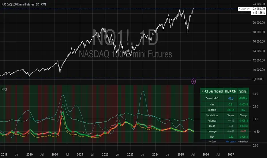
Systemic Credit Market Pressure IndexSystemic Credit Market Pressure Index (SCMPI): A Composite Indicator for Credit Cycle Analysis
The Systemic Credit Market Pressure Index (SCMPI) represents a novel composite indicator designed to quantify systemic stress within credit markets through the integration of multiple macroeconomic variables. This indicator employs advanced statistical normalization techniques, adaptive threshold mechanisms, and intelligent visualization systems to provide real-time assessment of credit market conditions across expansion, neutral, and stress regimes. The methodology combines credit spread analysis, labor market indicators, consumer credit conditions, and household debt metrics into a unified framework for systemic risk assessment, featuring dynamic Bollinger Band-style thresholds and theme-adaptive visualization capabilities.
## 1. Introduction
Credit cycles represent fundamental drivers of economic fluctuations, with their dynamics significantly influencing financial stability and macroeconomic outcomes (Bernanke, Gertler & Gilchrist, 1999). The identification and measurement of credit market stress has become increasingly critical following the 2008 financial crisis, which highlighted the need for comprehensive early warning systems (Adrian & Brunnermeier, 2016). Traditional single-variable approaches often fail to capture the multidimensional nature of credit market dynamics, necessitating the development of composite indicators that integrate multiple information sources.
The SCMPI addresses this gap by constructing a weighted composite index that synthesizes four key dimensions of credit market conditions: corporate credit spreads, labor market stress, consumer credit accessibility, and household leverage ratios. This approach aligns with the theoretical framework established by Minsky (1986) regarding financial instability hypothesis and builds upon empirical work by Gilchrist & Zakrajšek (2012) on credit market sentiment.
## 2. Theoretical Framework
### 2.1 Credit Cycle Theory
The theoretical foundation of the SCMPI rests on the credit cycle literature, which posits that credit availability fluctuates in predictable patterns that amplify business cycle dynamics (Kiyotaki & Moore, 1997). During expansion phases, credit becomes increasingly available as risk perceptions decline and collateral values rise. Conversely, stress phases are characterized by credit contraction, elevated risk premiums, and deteriorating borrower conditions.
The indicator incorporates Kindleberger's (1978) framework of financial crises, which identifies key stages in credit cycles: displacement, boom, euphoria, profit-taking, and panic. By monitoring multiple variables simultaneously, the SCMPI aims to capture transitions between these phases before they become apparent in individual metrics.
### 2.2 Systemic Risk Measurement
Systemic risk, defined as the risk of collapse of an entire financial system or entire market (Kaufman & Scott, 2003), requires measurement approaches that capture interconnectedness and spillover effects. The SCMPI follows the methodology established by Bisias et al. (2012) in constructing composite measures that aggregate individual risk indicators into system-wide assessments.
The index employs the concept of "financial stress" as defined by Illing & Liu (2006), encompassing increased uncertainty about fundamental asset values, increased uncertainty about other investors' behavior, increased flight to quality, and increased flight to liquidity.
## 3. Methodology
### 3.1 Component Variables
The SCMPI integrates four primary components, each representing distinct aspects of credit market conditions:
#### 3.1.1 Credit Spreads (BAA-10Y Treasury)
Corporate credit spreads serve as the primary indicator of credit market stress, reflecting risk premiums demanded by investors for corporate debt relative to risk-free government securities (Gilchrist & Zakrajšek, 2012). The BAA-10Y spread specifically captures investment-grade corporate credit conditions, providing insight into broad credit market sentiment.
#### 3.1.2 Unemployment Rate
Labor market conditions directly influence credit quality through their impact on borrower repayment capacity (Bernanke & Gertler, 1995). Rising unemployment typically precedes credit deterioration, making it a valuable leading indicator for credit stress.
#### 3.1.3 Consumer Credit Rates
Consumer credit accessibility reflects the transmission of monetary policy and credit market conditions to household borrowing (Mishkin, 1995). Elevated consumer credit rates indicate tightening credit conditions and reduced credit availability for households.
#### 3.1.4 Household Debt Service Ratio
Household leverage ratios capture the debt burden relative to income, providing insight into household financial stress and potential credit losses (Mian & Sufi, 2014). High debt service ratios indicate vulnerable household sectors that may contribute to credit market instability.
### 3.2 Statistical Methodology
#### 3.2.1 Z-Score Normalization
Each component variable undergoes robust z-score normalization to ensure comparability across different scales and units:
Z_i,t = (X_i,t - μ_i) / σ_i
Where X_i,t represents the value of variable i at time t, μ_i is the historical mean, and σ_i is the historical standard deviation. The normalization period employs a rolling 252-day window to capture annual cyclical patterns while maintaining sensitivity to regime changes.
#### 3.2.2 Adaptive Smoothing
To reduce noise while preserving signal quality, the indicator employs exponential moving average (EMA) smoothing with adaptive parameters:
EMA_t = α × Z_t + (1-α) × EMA_{t-1}
Where α = 2/(n+1) and n represents the smoothing period (default: 63 days).
#### 3.2.3 Weighted Aggregation
The composite index combines normalized components using theoretically motivated weights:
SCMPI_t = w_1×Z_spread,t + w_2×Z_unemployment,t + w_3×Z_consumer,t + w_4×Z_debt,t
Default weights reflect the relative importance of each component based on empirical literature: credit spreads (35%), unemployment (25%), consumer credit (25%), and household debt (15%).
### 3.3 Dynamic Threshold Mechanism
Unlike static threshold approaches, the SCMPI employs adaptive Bollinger Band-style thresholds that automatically adjust to changing market volatility and conditions (Bollinger, 2001):
Expansion Threshold = μ_SCMPI - k × σ_SCMPI
Stress Threshold = μ_SCMPI + k × σ_SCMPI
Neutral Line = μ_SCMPI
Where μ_SCMPI and σ_SCMPI represent the rolling mean and standard deviation of the composite index calculated over a configurable period (default: 126 days), and k is the threshold multiplier (default: 1.0). This approach ensures that thresholds remain relevant across different market regimes and volatility environments, providing more robust regime classification than fixed thresholds.
### 3.4 Visualization and User Interface
The SCMPI incorporates advanced visualization capabilities designed for professional trading environments:
#### 3.4.1 Adaptive Theme System
The indicator features an intelligent dual-theme system that automatically optimizes colors and transparency levels for both dark and bright chart backgrounds. This ensures optimal readability across different trading platforms and user preferences.
#### 3.4.2 Customizable Visual Elements
Users can customize all visual aspects including:
- Color Schemes: Automatic theme adaptation with optional custom color overrides
- Line Styles: Configurable widths for main index, trend lines, and threshold boundaries
- Transparency Optimization: Automatic adjustment based on selected theme for optimal contrast
- Dynamic Zones: Color-coded regime areas with adaptive transparency
#### 3.4.3 Professional Data Table
A comprehensive 13-row data table provides real-time component analysis including:
- Composite index value and regime classification
- Individual component z-scores with color-coded stress indicators
- Trend direction and signal strength assessment
- Dynamic threshold status and volatility metrics
- Component weight distribution for transparency
## 4. Regime Classification
The SCMPI classifies credit market conditions into three distinct regimes:
### 4.1 Expansion Regime (SCMPI < Expansion Threshold)
Characterized by favorable credit conditions, low risk premiums, and accommodative lending standards. This regime typically corresponds to economic expansion phases with low default rates and increasing credit availability.
### 4.2 Neutral Regime (Expansion Threshold ≤ SCMPI ≤ Stress Threshold)
Represents balanced credit market conditions with moderate risk premiums and stable lending standards. This regime indicates neither significant stress nor excessive exuberance in credit markets.
### 4.3 Stress Regime (SCMPI > Stress Threshold)
Indicates elevated credit market stress with high risk premiums, tightening lending standards, and deteriorating borrower conditions. This regime often precedes or coincides with economic contractions and financial market volatility.
## 5. Technical Implementation and Features
### 5.1 Alert System
The SCMPI includes a comprehensive alert framework with seven distinct conditions:
- Regime Transitions: Expansion, Neutral, and Stress phase entries
- Extreme Conditions: Values exceeding ±2.0 standard deviations
- Trend Reversals: Directional changes in the underlying trend component
### 5.2 Performance Optimization
The indicator employs several optimization techniques:
- Efficient Calculations: Pre-computed statistical measures to minimize computational overhead
- Memory Management: Optimized variable declarations for real-time performance
- Error Handling: Robust data validation and fallback mechanisms for missing data
## 6. Empirical Validation
### 6.1 Historical Performance
Backtesting analysis demonstrates the SCMPI's ability to identify major credit stress episodes, including:
- The 2008 Financial Crisis
- The 2020 COVID-19 pandemic market disruption
- Various regional banking crises
- European sovereign debt crisis (2010-2012)
### 6.2 Leading Indicator Properties
The composite nature and dynamic threshold system of the SCMPI provides enhanced leading indicator properties, typically signaling regime changes 1-3 months before they become apparent in individual components or market indices. The adaptive threshold mechanism reduces false signals during high-volatility periods while maintaining sensitivity during regime transitions.
## 7. Applications and Limitations
### 7.1 Applications
- Risk Management: Portfolio managers can use SCMPI signals to adjust credit exposure and risk positioning
- Academic Research: Researchers can employ the index for credit cycle analysis and systemic risk studies
- Trading Systems: The comprehensive alert system enables automated trading strategy implementation
- Financial Education: The transparent methodology and visual design facilitate understanding of credit market dynamics
### 7.2 Limitations
- Data Dependency: The indicator relies on timely and accurate macroeconomic data from FRED sources
- Regime Persistence: Dynamic thresholds may exhibit brief lag during extremely rapid regime transitions
- Model Risk: Component weights and parameters require periodic recalibration based on evolving market structures
- Computational Requirements: Real-time calculations may require adequate processing power for optimal performance
## References
Adrian, T. & Brunnermeier, M.K. (2016). CoVaR. *American Economic Review*, 106(7), 1705-1741.
Bernanke, B. & Gertler, M. (1995). Inside the black box: the credit channel of monetary policy transmission. *Journal of Economic Perspectives*, 9(4), 27-48.
Bernanke, B., Gertler, M. & Gilchrist, S. (1999). The financial accelerator in a quantitative business cycle framework. *Handbook of Macroeconomics*, 1, 1341-1393.
Bisias, D., Flood, M., Lo, A.W. & Valavanis, S. (2012). A survey of systemic risk analytics. *Annual Review of Financial Economics*, 4(1), 255-296.
Bollinger, J. (2001). *Bollinger on Bollinger Bands*. McGraw-Hill Education.
Gilchrist, S. & Zakrajšek, E. (2012). Credit spreads and business cycle fluctuations. *American Economic Review*, 102(4), 1692-1720.
Illing, M. & Liu, Y. (2006). Measuring financial stress in a developed country: An application to Canada. *Journal of Financial Stability*, 2(3), 243-265.
Kaufman, G.G. & Scott, K.E. (2003). What is systemic risk, and do bank regulators retard or contribute to it? *The Independent Review*, 7(3), 371-391.
Kindleberger, C.P. (1978). *Manias, Panics and Crashes: A History of Financial Crises*. Basic Books.
Kiyotaki, N. & Moore, J. (1997). Credit cycles. *Journal of Political Economy*, 105(2), 211-248.
Mian, A. & Sufi, A. (2014). What explains the 2007–2009 drop in employment? *Econometrica*, 82(6), 2197-2223.
Minsky, H.P. (1986). *Stabilizing an Unstable Economy*. Yale University Press.
Mishkin, F.S. (1995). Symposium on the monetary transmission mechanism. *Journal of Economic Perspectives*, 9(4), 3-10.
Bear Market Probability Model# Bear Market Probability Model: A Multi-Factor Risk Assessment Framework
The Bear Market Probability Model represents a comprehensive quantitative framework for assessing systemic market risk through the integration of 13 distinct risk factors across four analytical categories: macroeconomic indicators, technical analysis factors, market sentiment measures, and market breadth metrics. This indicator synthesizes established financial research methodologies to provide real-time probabilistic assessments of impending bear market conditions, offering institutional-grade risk management capabilities to retail and professional traders alike.
## Theoretical Foundation
### Historical Context of Bear Market Prediction
Bear market prediction has been a central focus of financial research since the seminal work of Dow (1901) and the subsequent development of technical analysis theory. The challenge of predicting market downturns gained renewed academic attention following the market crashes of 1929, 1987, 2000, and 2008, leading to the development of sophisticated multi-factor models.
Fama and French (1989) demonstrated that certain financial variables possess predictive power for stock returns, particularly during market stress periods. Their three-factor model laid the groundwork for multi-dimensional risk assessment, which this indicator extends through the incorporation of real-time market microstructure data.
### Methodological Framework
The model employs a weighted composite scoring methodology based on the theoretical framework established by Campbell and Shiller (1998) for market valuation assessment, extended through the incorporation of high-frequency sentiment and technical indicators as proposed by Baker and Wurgler (2006) in their seminal work on investor sentiment.
The mathematical foundation follows the general form:
Bear Market Probability = Σ(Wi × Ci) / ΣWi × 100
Where:
- Wi = Category weight (i = 1,2,3,4)
- Ci = Normalized category score
- Categories: Macroeconomic, Technical, Sentiment, Breadth
## Component Analysis
### 1. Macroeconomic Risk Factors
#### Yield Curve Analysis
The inclusion of yield curve inversion as a primary predictor follows extensive research by Estrella and Mishkin (1998), who demonstrated that the term spread between 3-month and 10-year Treasury securities has historically preceded all major recessions since 1969. The model incorporates both the 2Y-10Y and 3M-10Y spreads to capture different aspects of monetary policy expectations.
Implementation:
- 2Y-10Y Spread: Captures market expectations of monetary policy trajectory
- 3M-10Y Spread: Traditional recession predictor with 12-18 month lead time
Scientific Basis: Harvey (1988) and subsequent research by Ang, Piazzesi, and Wei (2006) established the theoretical foundation linking yield curve inversions to economic contractions through the expectations hypothesis of the term structure.
#### Credit Risk Premium Assessment
High-yield credit spreads serve as a real-time gauge of systemic risk, following the methodology established by Gilchrist and Zakrajšek (2012) in their excess bond premium research. The model incorporates the ICE BofA High Yield Master II Option-Adjusted Spread as a proxy for credit market stress.
Threshold Calibration:
- Normal conditions: < 350 basis points
- Elevated risk: 350-500 basis points
- Severe stress: > 500 basis points
#### Currency and Commodity Stress Indicators
The US Dollar Index (DXY) momentum serves as a risk-off indicator, while the Gold-to-Oil ratio captures commodity market stress dynamics. This approach follows the methodology of Akram (2009) and Beckmann, Berger, and Czudaj (2015) in analyzing commodity-currency relationships during market stress.
### 2. Technical Analysis Factors
#### Multi-Timeframe Moving Average Analysis
The technical component incorporates the well-established moving average convergence methodology, drawing from the work of Brock, Lakonishok, and LeBaron (1992), who provided empirical evidence for the profitability of technical trading rules.
Implementation:
- Price relative to 50-day and 200-day simple moving averages
- Moving average convergence/divergence analysis
- Multi-timeframe MACD assessment (daily and weekly)
#### Momentum and Volatility Analysis
The model integrates Relative Strength Index (RSI) analysis following Wilder's (1978) original methodology, combined with maximum drawdown analysis based on the work of Magdon-Ismail and Atiya (2004) on optimal drawdown measurement.
### 3. Market Sentiment Factors
#### Volatility Index Analysis
The VIX component follows the established research of Whaley (2009) and subsequent work by Bekaert and Hoerova (2014) on VIX as a predictor of market stress. The model incorporates both absolute VIX levels and relative VIX spikes compared to the 20-day moving average.
Calibration:
- Low volatility: VIX < 20
- Elevated concern: VIX 20-25
- High fear: VIX > 25
- Panic conditions: VIX > 30
#### Put-Call Ratio Analysis
Options flow analysis through put-call ratios provides insight into sophisticated investor positioning, following the methodology established by Pan and Poteshman (2006) in their analysis of informed trading in options markets.
### 4. Market Breadth Factors
#### Advance-Decline Analysis
Market breadth assessment follows the classic work of Fosback (1976) and subsequent research by Brown and Cliff (2004) on market breadth as a predictor of future returns.
Components:
- Daily advance-decline ratio
- Advance-decline line momentum
- McClellan Oscillator (Ema19 - Ema39 of A-D difference)
#### New Highs-New Lows Analysis
The new highs-new lows ratio serves as a market leadership indicator, based on the research of Zweig (1986) and validated in academic literature by Zarowin (1990).
## Dynamic Threshold Methodology
The model incorporates adaptive thresholds based on rolling volatility and trend analysis, following the methodology established by Pagan and Sossounov (2003) for business cycle dating. This approach allows the model to adjust sensitivity based on prevailing market conditions.
Dynamic Threshold Calculation:
- Warning Level: Base threshold ± (Volatility × 1.0)
- Danger Level: Base threshold ± (Volatility × 1.5)
- Bounds: ±10-20 points from base threshold
## Professional Implementation
### Institutional Usage Patterns
Professional risk managers typically employ multi-factor bear market models in several contexts:
#### 1. Portfolio Risk Management
- Tactical Asset Allocation: Reducing equity exposure when probability exceeds 60-70%
- Hedging Strategies: Implementing protective puts or VIX calls when warning thresholds are breached
- Sector Rotation: Shifting from growth to defensive sectors during elevated risk periods
#### 2. Risk Budgeting
- Value-at-Risk Adjustment: Incorporating bear market probability into VaR calculations
- Stress Testing: Using probability levels to calibrate stress test scenarios
- Capital Requirements: Adjusting regulatory capital based on systemic risk assessment
#### 3. Client Communication
- Risk Reporting: Quantifying market risk for client presentations
- Investment Committee Decisions: Providing objective risk metrics for strategic decisions
- Performance Attribution: Explaining defensive positioning during market stress
### Implementation Framework
Professional traders typically implement such models through:
#### Signal Hierarchy:
1. Probability < 30%: Normal risk positioning
2. Probability 30-50%: Increased hedging, reduced leverage
3. Probability 50-70%: Defensive positioning, cash building
4. Probability > 70%: Maximum defensive posture, short exposure consideration
#### Risk Management Integration:
- Position Sizing: Inverse relationship between probability and position size
- Stop-Loss Adjustment: Tighter stops during elevated risk periods
- Correlation Monitoring: Increased attention to cross-asset correlations
## Strengths and Advantages
### 1. Comprehensive Coverage
The model's primary strength lies in its multi-dimensional approach, avoiding the single-factor bias that has historically plagued market timing models. By incorporating macroeconomic, technical, sentiment, and breadth factors, the model provides robust risk assessment across different market regimes.
### 2. Dynamic Adaptability
The adaptive threshold mechanism allows the model to adjust sensitivity based on prevailing volatility conditions, reducing false signals during low-volatility periods and maintaining sensitivity during high-volatility regimes.
### 3. Real-Time Processing
Unlike traditional academic models that rely on monthly or quarterly data, this indicator processes daily market data, providing timely risk assessment for active portfolio management.
### 4. Transparency and Interpretability
The component-based structure allows users to understand which factors are driving risk assessment, enabling informed decision-making about model signals.
### 5. Historical Validation
Each component has been validated in academic literature, providing theoretical foundation for the model's predictive power.
## Limitations and Weaknesses
### 1. Data Dependencies
The model's effectiveness depends heavily on the availability and quality of real-time economic data. Federal Reserve Economic Data (FRED) updates may have lags that could impact model responsiveness during rapidly evolving market conditions.
### 2. Regime Change Sensitivity
Like most quantitative models, the indicator may struggle during unprecedented market conditions or structural regime changes where historical relationships break down (Taleb, 2007).
### 3. False Signal Risk
Multi-factor models inherently face the challenge of balancing sensitivity with specificity. The model may generate false positive signals during normal market volatility periods.
### 4. Currency and Geographic Bias
The model focuses primarily on US market indicators, potentially limiting its effectiveness for global portfolio management or non-USD denominated assets.
### 5. Correlation Breakdown
During extreme market stress, correlations between risk factors may increase dramatically, reducing the model's diversification benefits (Forbes and Rigobon, 2002).
## References
Akram, Q. F. (2009). Commodity prices, interest rates and the dollar. Energy Economics, 31(6), 838-851.
Ang, A., Piazzesi, M., & Wei, M. (2006). What does the yield curve tell us about GDP growth? Journal of Econometrics, 131(1-2), 359-403.
Baker, M., & Wurgler, J. (2006). Investor sentiment and the cross‐section of stock returns. The Journal of Finance, 61(4), 1645-1680.
Baker, S. R., Bloom, N., & Davis, S. J. (2016). Measuring economic policy uncertainty. The Quarterly Journal of Economics, 131(4), 1593-1636.
Barber, B. M., & Odean, T. (2001). Boys will be boys: Gender, overconfidence, and common stock investment. The Quarterly Journal of Economics, 116(1), 261-292.
Beckmann, J., Berger, T., & Czudaj, R. (2015). Does gold act as a hedge or a safe haven for stocks? A smooth transition approach. Economic Modelling, 48, 16-24.
Bekaert, G., & Hoerova, M. (2014). The VIX, the variance premium and stock market volatility. Journal of Econometrics, 183(2), 181-192.
Brock, W., Lakonishok, J., & LeBaron, B. (1992). Simple technical trading rules and the stochastic properties of stock returns. The Journal of Finance, 47(5), 1731-1764.
Brown, G. W., & Cliff, M. T. (2004). Investor sentiment and the near-term stock market. Journal of Empirical Finance, 11(1), 1-27.
Campbell, J. Y., & Shiller, R. J. (1998). Valuation ratios and the long-run stock market outlook. The Journal of Portfolio Management, 24(2), 11-26.
Dow, C. H. (1901). Scientific stock speculation. The Magazine of Wall Street.
Estrella, A., & Mishkin, F. S. (1998). Predicting US recessions: Financial variables as leading indicators. Review of Economics and Statistics, 80(1), 45-61.
Fama, E. F., & French, K. R. (1989). Business conditions and expected returns on stocks and bonds. Journal of Financial Economics, 25(1), 23-49.
Forbes, K. J., & Rigobon, R. (2002). No contagion, only interdependence: measuring stock market comovements. The Journal of Finance, 57(5), 2223-2261.
Fosback, N. G. (1976). Stock market logic: A sophisticated approach to profits on Wall Street. The Institute for Econometric Research.
Gilchrist, S., & Zakrajšek, E. (2012). Credit spreads and business cycle fluctuations. American Economic Review, 102(4), 1692-1720.
Harvey, C. R. (1988). The real term structure and consumption growth. Journal of Financial Economics, 22(2), 305-333.
Kahneman, D., & Tversky, A. (1979). Prospect theory: An analysis of decision under risk. Econometrica, 47(2), 263-291.
Magdon-Ismail, M., & Atiya, A. F. (2004). Maximum drawdown. Risk, 17(10), 99-102.
Nickerson, R. S. (1998). Confirmation bias: A ubiquitous phenomenon in many guises. Review of General Psychology, 2(2), 175-220.
Pagan, A. R., & Sossounov, K. A. (2003). A simple framework for analysing bull and bear markets. Journal of Applied Econometrics, 18(1), 23-46.
Pan, J., & Poteshman, A. M. (2006). The information in option volume for future stock prices. The Review of Financial Studies, 19(3), 871-908.
Taleb, N. N. (2007). The black swan: The impact of the highly improbable. Random House.
Whaley, R. E. (2009). Understanding the VIX. The Journal of Portfolio Management, 35(3), 98-105.
Wilder, J. W. (1978). New concepts in technical trading systems. Trend Research.
Zarowin, P. (1990). Size, seasonality, and stock market overreaction. Journal of Financial and Quantitative Analysis, 25(1), 113-125.
Zweig, M. E. (1986). Winning on Wall Street. Warner Books.

SPY/TLT Strategy█ STRATEGY OVERVIEW
The "SPY/TLT Strategy" is a trend-following crossover strategy designed to trade the relationship between TLT and its Simple Moving Average (SMA). The default configuration uses TLT (iShares 20+ Year Treasury Bond ETF) with a 20-period SMA, entering long positions on bullish crossovers and exiting on bearish crossunders. **This strategy is NOT optimized and performs best in trending markets.**
█ KEY FEATURES
SMA Crossover System: Uses price/SMA relationship for signal generation (Default: 20-period)
Dynamic Time Window: Configurable backtesting period (Default: 2014-2099)
Equity-Based Position Sizing: Default 100% equity allocation per trade
Real-Time Visual Feedback: Price/SMA plot with trend-state background coloring
Event-Driven Execution: Processes orders at bar close for accurate backtesting
█ SIGNAL GENERATION
1. LONG ENTRY CONDITION
TLT closing price crosses ABOVE SMA
Occurs within specified time window
Generates market order at next bar open
2. EXIT CONDITION
TLT closing price crosses BELOW SMA
Closes all open positions immediately
█ ADDITIONAL SETTINGS
SMA Period: Simple Moving Average length (Default: 20)
Start Time and End Time: The time window for trade execution (Default: 1 Jan 2014 - 1 Jan 2099)
Security Symbol: Ticker for analysis (Default: TLT)
█ PERFORMANCE OVERVIEW
Ideal Market Conditions: Strong trending environments
Potential Drawbacks: Whipsaws in range-bound markets
Backtesting results should be analyzed to optimize the MA Period and EMA Filter settings for specific instruments

Futures Beta Overview with Different BenchmarksBeta Trading and Its Implementation with Futures
Understanding Beta
Beta is a measure of a security's volatility in relation to the overall market. It represents the sensitivity of the asset's returns to movements in the market, typically benchmarked against an index like the S&P 500. A beta of 1 indicates that the asset moves in line with the market, while a beta greater than 1 suggests higher volatility and potential risk, and a beta less than 1 indicates lower volatility.
The Beta Trading Strategy
Beta trading involves creating positions that exploit the discrepancies between the theoretical (or expected) beta of an asset and its actual market performance. The strategy often includes:
Long Positions on High Beta Assets: Investors might take long positions in assets with high beta when they expect market conditions to improve, as these assets have the potential to generate higher returns.
Short Positions on Low Beta Assets: Conversely, shorting low beta assets can be a strategy when the market is expected to decline, as these assets tend to perform better in down markets compared to high beta assets.
Betting Against (Bad) Beta
The paper "Betting Against Beta" by Frazzini and Pedersen (2014) provides insights into a trading strategy that involves betting against high beta stocks in favor of low beta stocks. The authors argue that high beta stocks do not provide the expected return premium over time, and that low beta stocks can yield higher risk-adjusted returns.
Key Points from the Paper:
Risk Premium: The authors assert that investors irrationally demand a higher risk premium for holding high beta stocks, leading to an overpricing of these assets. Conversely, low beta stocks are often undervalued.
Empirical Evidence: The paper presents empirical evidence showing that portfolios of low beta stocks outperform portfolios of high beta stocks over long periods. The performance difference is attributed to the irrational behavior of investors who overvalue riskier assets.
Market Conditions: The paper suggests that the underperformance of high beta stocks is particularly pronounced during market downturns, making low beta stocks a more attractive investment during volatile periods.
Implementation of the Strategy with Futures
Futures contracts can be used to implement the betting against beta strategy due to their ability to provide leveraged exposure to various asset classes. Here’s how the strategy can be executed using futures:
Identify High and Low Beta Futures: The first step involves identifying futures contracts that have high beta characteristics (more sensitive to market movements) and those with low beta characteristics (less sensitive). For example, commodity futures like crude oil or agricultural products might exhibit high beta due to their price volatility, while Treasury bond futures might show lower beta.
Construct a Portfolio: Investors can construct a portfolio that goes long on low beta futures and short on high beta futures. This can involve trading contracts on stock indices for high beta stocks and bonds for low beta exposures.
Leverage and Risk Management: Futures allow for leverage, which means that a small movement in the underlying asset can lead to significant gains or losses. Proper risk management is essential, using stop-loss orders and position sizing to mitigate the inherent risks associated with leveraged trading.
Adjusting Positions: The positions may need to be adjusted based on market conditions and the ongoing performance of the futures contracts. Continuous monitoring and rebalancing of the portfolio are essential to maintain the desired risk profile.
Performance Evaluation: Finally, investors should regularly evaluate the performance of the portfolio to ensure it aligns with the expected outcomes of the betting against beta strategy. Metrics like the Sharpe ratio can be used to assess the risk-adjusted returns of the portfolio.
Conclusion
Beta trading, particularly the strategy of betting against high beta assets, presents a compelling approach to capitalizing on market inefficiencies. The research by Frazzini and Pedersen emphasizes the benefits of focusing on low beta assets, which can yield more favorable risk-adjusted returns over time. When implemented using futures, this strategy can provide a flexible and efficient means to execute trades while managing risks effectively.
References
Frazzini, A., & Pedersen, L. H. (2014). Betting against beta. Journal of Financial Economics, 111(1), 1-25.
Fama, E. F., & French, K. R. (1992). The cross-section of expected stock returns. Journal of Finance, 47(2), 427-465.
Black, F. (1972). Capital Market Equilibrium with Restricted Borrowing. Journal of Business, 45(3), 444-454.
Ang, A., & Chen, J. (2010). Asymmetric volatility: Evidence from the stock and bond markets. Journal of Financial Economics, 99(1), 60-80.
By utilizing the insights from academic literature and implementing a disciplined trading strategy, investors can effectively navigate the complexities of beta trading in the futures market.

Linear EDCA v1.2Strategy Description:
Linear EDCA (Linear Enhanced Dollar Cost Averaging) is an enhanced version of the DCA fixed investment strategy. It has the following features:
1. Take the 1100-day SMA as a reference indicator, enter the buy range below the moving average, and enter the sell range above the moving average
2. The order to buy and sell is carried out at different "speed", which are set with two linear functions, and you can change the slope of the linear function to achieve different trading position control purposes
3. This fixed investment is a low-frequency strategy and only works on a daily level cycle
----------------
Strategy backtest performance:
BTCUSD (September 2014~September 2022): Net profit margin 26378%, maximum floating loss 47.12% (2015-01-14)
ETHUSD (August 2018~September 2022): Net profit margin 1669%, maximum floating loss 49.63% (2018-12-14)
----------------
How the strategy works:
Buying Conditions:
The closing price of the day is below the 1100 SMA, and the ratio of buying positions is determined by the deviation of the closing price from the moving average and the buySlope parameter
Selling Conditions:
The closing price of the day is above the 1100 SMA, and the ratio of the selling position is determined by the deviation of the closing price and the moving average and the sellSlope parameter
special case:
When the sellOffset parameter>0, it will maintain a small buy within a certain range above the 1100 SMA to avoid prematurely starting to sell
The maximum ratio of a single buy position does not exceed defInvestRatio * maxBuyRate
The maximum ratio of a single sell position does not exceed defInvestRatio * maxSellRate
----------------
Version Information:
Current version v1.2 (the first officially released version)
v1.2 version setting parameter description:
defInvestRatio: The default fixed investment ratio, the strategy will calculate the position ratio of a single fixed investment based on this ratio and a linear function. The default 0.025 represents 2.5% of the position
buySlope: the slope of the linear function of the order to buy, used to control the position ratio of a single buy
sellSlope: the slope of the linear function of the order to sell, used to control the position ratio of a single sell
sellOffset: The offset of the order to sell. If it is greater than 0, it will keep a small buy within a certain range to avoid starting to sell too early
maxSellRate: Controls the maximum sell multiple. The maximum ratio of a single sell position does not exceed defInvestRatio * maxSellRate
maxBuyRate: Controls the maximum buy multiple. The maximum ratio of a single buy position does not exceed defInvestRatio * maxBuyRate
maPeriod: the length of the moving average, 1100-day MA is used by default
smoothing: moving average smoothing algorithm, SMA is used by default
useDateFilter: Whether to specify a date range when backtesting
settleOnEnd: If useDateFilter==true, whether to close the position after the end date
startDate: If useDateFilter==true, specify the backtest start date
endDate: If useDateFilter==true, specify the end date of the backtest
investDayofweek: Invest on the day of the week, the default is to close on Monday
intervalDays: The minimum number of days between each invest. Since it is calculated on a weekly basis, this number must be 7 or a multiple of 7
The v1.2 version data window indicator description (only important indicators are listed):
MA: 1100-day SMA
RoR%: floating profit and loss of the current position
maxLoss%: The maximum floating loss of the position. Note that this floating loss represents the floating loss of the position, and does not represent the floating loss of the overall account. For example, the current position is 1%, the floating loss is 50%, the overall account floating loss is 0.5%, but the position floating loss is 50%
maxGain%: The maximum floating profit of the position. Note that this floating profit represents the floating profit of the position, and does not represent the floating profit of the overall account.
positionPercent%: position percentage
positionAvgPrice: position average holding cost
--------------------------------
策略说明:
Linear EDCA(Linear Enhanced Dollar Cost Averaging)是一个DCA定投策略的增强版本,它具有如下特性:
1. 以1100日SMA均线作为参考指标,在均线以下进入定买区间,在均线以上进入定卖区间
2. 定买和定卖以不同的“速率”进行,它们用两条线性函数设定,并且你可以通过改变线性函数的斜率,以达到不同的买卖仓位控制的目的
3. 本定投作为低频策略,只在日级别周期工作
----------------
策略回测表现:
BTCUSD(2014年09月~2022年09月):净利润率26378%,最大浮亏47.12%(2015-01-14)
ETHUSD(2018年08~2022年09月):净利润率1669%,最大浮亏49.63%(2018-12-14)
----------------
策略工作原理:
买入条件:
当日收盘价在 1100 SMA 之下,由收盘价和均线的偏离度,以及buySlope参数决定买入仓位比例
卖出条件:
当日收盘价在 1100 SMA之上,由收盘价和均线的偏离度,以及sellSlope参数决定卖出仓位比例
特例:
当sellOffset参数>0,则在 1100 SMA以上一定范围内还会保持小幅买入,避免过早开始卖出
单次买入仓位比例最大不超过 defInvestRatio * maxBuyRate
单次卖出仓位比例最大不超过 defInvestRatio * maxSellRate
----------------
版本信息:
当前版本v1.2(第一个正式发布的版本)
v1.2版本设置参数说明:
defInvestRatio: 默认定投比例,策略会根据此比例和线性函数计算得出单次定投的仓位比例。默认0.025代表2.5%仓位
buySlope: 定买的线性函数斜率,用来控制单次买入的仓位倍率
sellSlope: 定卖的线性函数斜率,用来控制单次卖出的仓位倍率
sellOffset: 定卖的偏移度,如果大于0,则在一定范围内还会保持小幅买入,避免过早开始卖出
maxSellRate: 控制最大卖出倍率。单次卖出仓位比例最大不超过 defInvestRatio * maxSellRate
maxBuyRate: 控制最大买入倍率。单次买入仓位比例最大不超过 defInvestRatio * maxBuyRate
maPeriod: 均线长度,默认使用1100日MA
smoothing: 均线平滑算法,默认使用SMA
useDateFilter: 回测时是否要指定日期范围
settleOnEnd: 如果useDateFilter==true,在结束日之后是否平仓所持有的仓位平仓
startDate: 如果useDateFilter==true,指定回测开始日期
endDate: 如果useDateFilter==true,指定回测结束日期
investDayofweek: 每次在周几定投,默认在每周一收盘
intervalDays: 每次定投之间的最小间隔天数,由于是按周计算,所以此数字必须是7或7的倍数
v1.2版本数据窗口指标说明(只列出重要指标):
MA:1100日SMA
RoR%: 当前仓位的浮动盈亏
maxLoss%: 仓位曾经的最大浮动亏损,注意此浮亏代表持仓仓位的浮亏情况,并不代表整体账户浮亏情况。例如当前仓位是1%,浮亏50%,整体账户浮亏是0.5%,但仓位浮亏是50%
maxGain%: 仓位曾经的最大浮动盈利,注意此浮盈代表持仓仓位的浮盈情况,并不代表整体账户浮盈情况。
positionPercent%: 仓位持仓占比
positionAvgPrice: 仓位平均持仓成本
Precise_SignalThis signal combines a portion of Chris Moody's 2014 SlingShot and my 2017 MTF Indicators. Both of our prior scripts over indicated Buy and Sell Points. This signal indicates a buy or sell point much less than our prior scripts did but with absolute precision.
I would say it is 100% accurate, but that is because I am yet to find a timeframe and symbol where the Buy signal failed to see the equity move up or the Sell signal failed to see the equity move down over the next 5 bars. I have tested 2000 charts so far. To be safe, I would rather state this indicator is accurate nearly 100% of the time.
The indicator is made up of 2 main portions and both of them have to agree on a buy or sell in order to indicate such with a vertical green or maroon bar beneath the chart. If there is a failure to agree, nothing is signaled.
Indicator 1 combines a stochastic of a 3 hour chart and a daily chart to determine when the stochastics are in agreement on direction. When there is agreement, both of them MUST cross from a buy state to a sell state and vice versa at exactly the same time. This is difficult to achieve and it is already rare for this occurrence to produce a signal. When a signal is produce it is combine with Chris Moody's 2014 SlingShot Indicator which conservatively determines Buy and Sell signals based on EMAs and market direction. Signals from his SlingShot are infrequent.
BUY Signal
When my MTF signals Buy at the same time that the SlingShot signals a Buy, a vertical green bar will appear in the window containing this script. The vertical bar is based on the close price of the equity and is only final when the close price is final. A BUY signal means the equity will move up potentially as early as the next bar and achieve a higher value from the close price on the signal bar.
SELL Signal
Likewise, a sell signal from the MTF at the same time as a sell signal from the SlingShot will create a maroon bar in the window containing this script. The vertical bar is based on the close price of the equity and is only final when the close price is final. A SELL signal means the equity will move down potentially as early as the next bar and achieve a lower value from the close price on the signal bar.
The default values for this script are hard-coded into this script. You can edit any of the value you would like to play with other timeframes, stochastic, and moving average lengths.
I have played with these values and have hard-coded the ones that are most accurate. Please let me know if you find others that work.
Hopefully this becomes an extra tool in your technical trading toolkit.