McGinley Dynamic VWAP/MVWAP [Dayasagar]Mcginley Dynamics and Volume weighted moving average
Timeframe: 1 hour
Use 200 MA
Buy: If the price is above 200 MA, take only the buy signal.
Sell: If the price is below 200 MA, take only the sell signal.
Wyszukaj w skryptach "200亿美元是多少人民币"

7EMA_5MA (G/D + Bias + 12/26 Signal)This script alow you to survey multiple crossing signals as Golden/Death cross (MA50/200), Institutional Bias (EMA9/18), or EMA 12/26 crossing. You can show/hide all EMAs/MAs and show/hide all signals. Default config displays EMA 50/100/200 and MA 20. Full script includes display of EMA 9/18/12/26/50/100/200 and MA 20/21/50/100/200.

Sequentially Filtered Moving AverageThe previously proposed sequential filter aimed to filter variations lower than a certain period, this allowed to remove noisy variations and retain only the closing price values that occurred after a consecutive up/down, however because of the noisy nature of the closing price large filtering was impossible, in order to tackle to this problem the same indicator using a simple moving average as input is proposed, this allow for smoother results.
We will see that the proposed indicator can provide an alternative moving average that could be used as slow moving average in crossover systems.
The Indicator
The length parameter as the same function as the one described in the sequential filter post, however here length also control the period of the moving average used input, in short larger values of length will return a smoother but less reactive output.
In blue the moving average with length = 200, and in red the moving average with length = 50.
It is interesting to see how the moving average remain flat during ranging/flat market periods
Unfortunately like the sequential filter the sequentially filtered moving average (SFMA) is not affected by large short term variations such as gaps or short term volatile events. This is because of the nature of the sequential filter to ignore movements amplitude and only focus on the variation period.
Moving Average Crossover System
The SFMA is equal to a simple moving average of period length when a consecutive up/down sequence of size length has occurred, else the SFMA is equal to its precedent value, therefore we could expect less crosses between a fast moving average and the SFMA as slow moving average.
We can see on the figure above that the fast moving average of period 50 (in green) cross more with the slow moving average of period 200 (in red) than with the SFMA of period 200 (in blue).
Crosses can occur at the same time as with the classical slow moving average (in red) or a bit later.
Conclusion
A new moving average based on the recently proposed sequential filter has been proposed, it can be seen that under a moving average crossover system the proposed moving average seems to be more effective at producing less crosses without necessarily doing it with an excessive lag, in fact the moving average has either lag (length-1)/2 or lag length .
In the future it could be interesting to provide an hybrid alternative that take into account volatility as well as variations period.
Thanks for reading !

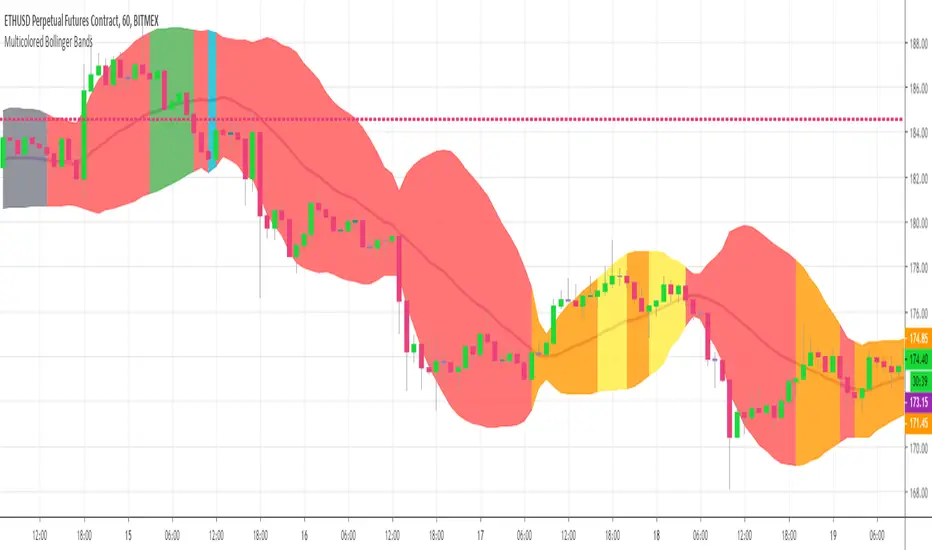
Multicolor Bollinger Bands - Market PhasesHi everyone
Hope you're all doing well 😘
Today I feel gracious and decided to give to the community. And giving not only an indicator but also a trading method
This trading method shows how a convergence based on moving averages is tremendous
Multicolour Bollinger Bands indicator that indicates market phases.
It plots on the price chart, thanks to different color zones between the bands, a breakdown of the different phases that the price operates during a trend.
The different zones are identified as follows:
- red color zone: trend is bearish, price is below the 200 periods moving average
- orange color zone: price operate a technical rebound below the 200 periods moving average
- yellow color zone: (phase 1 which indicate a new bearish cycle)
- light green zone: (phase 2 which indicate a new bullish cycle)
- dark green zone: trend is bullish, price is above the 200 periods moving average
- grey color zone: calm phase of price
- dark blue color zone: price is consolidating in either bullish or bearish trend
- light blue zones: price will revert to a new opposite trend (either long or short new trend)
By identifying clearly the different market phases with the multicolor Bollinger bands, the market entries by either a the beginning of a new trend or just after a rebound or a consolidating phase is easier to spot on.
Trade well and trade safe
Dave
EMA - Baby WhaleThis script will show you the 8, 13, 21, 55, 100 and 200 EMA .
You can change the colors yourself if you want.
You can use the EMA to define the trend.
A good strategy that traders use is a 55 EMA crossover.
This means that when the 8, 13 and 21 all cross the 55 EMA you place a buy or sell order.
You close your position when the same thing happens on the other side.
Another great way that traders use these EMA's is to spot a Golden or Death cross.
When the 55 and 200 EMA cross and the 200 becomes support it means we're in a uptrend and vice versa.
If you want access, just send a message please.
Much love from Baby Whale!!
🙏❤️🐳

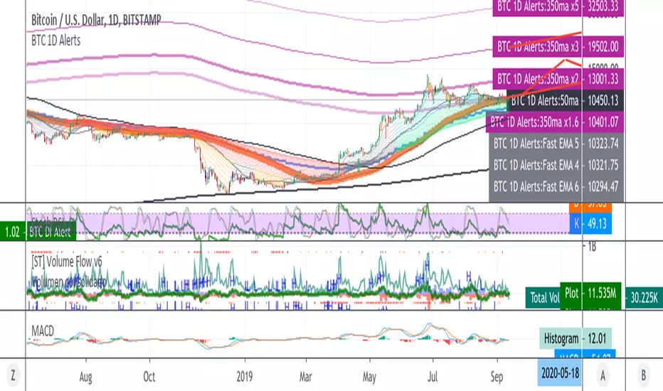
BTC 1D Alerts V1This script contains a variety of key indicator for bitcoin all-in-one and they can be activated individually in the menu. These are meant to be used on the 1D chart for Bitcoin.
1457 Day Moving Average: the bottom of the bitcoin price and arguably the rock bottom price target.
Ichimoku Cloud: a common useful indicator for bitcoin support and resistance.
350ma fibs (21 8 5 3 2 and 1.6) : Signify the tops of each logarthmic rise in bitcoin price. They are generally curving higher over the long term. For halvening #3, the predicted market crash would be after hitting the 350ma x3 fib. Also the 350 ma / 111 ma cross signifies bull market top within about 3 days as well. Using the combination of the 350ma fibs and the 350/111 crosses, reasonably identify when market top is about to occur.
50,120,200 ma: Common moving averages that bitcoin retests during bull market runs. Also, the 50/200 golden and death crosses.
1D EMA Superguppy Ribbons: green = bull market, gray is indeterminate, red = bear market. Very high specificity indicator of bull runs, especially for bitcoin. You can change to 3D candle for even more specificity for a bull market start. Use the 1W for even more specificity. 1D Superguppy is recommended for decisionmaking.
1W EMA21: a very good moving average programmed to be shown on both the daily and weekly candle time. Bitcoin commonly corrects to this repeatedly during past bull runs. Acts as support during bull run and resistance during a bear market.
Steps to identifying a bull market:
1. 50/200 golden cross
2. 1D EMA superguppy green
3. 3D EMA superguppy green (if you prefer more certainty than step 2).
4. Hitting the 1W EMA21 and bouncing off during the bull run signifies corrections.
Once a bull market is identified,
Additional recommended buying and selling techniques:
Indicators:
- Fiblines - to determine retracements from peaks (such as all time high or recent highs)
- Stochastic RSI - 1d, 3d, and 1W SRSI are great time to buy, especially the 1W SRSI which comes much less frequently.
- volumen consolidado - for multi exchange volumes compiled into a single line. I prefer buying on the lowest volume days which generally coincide with dips.
- MACD - somewhat dubious utility but many algorithms are programmed to buy or sell based on this.
Check out the Alerts for golden crosses and 350ma Fib crosses which are invaluable for long term buying planning.
I left this open source so that all the formulas can be understood and verified. Much of it hacked together from other sources but all indicators that are fundamental to bitcoin. I apologize in advance for not attributing all the articles and references... but then again I am making no money off of this anyway.
Ultimate Moving Average Package (17 MA's)Included is the:
VWAP
Current time frame 10 EMA
Current time frame 20 EMA
Current time frame 50 EMA
Current time frame 10 SMA
Current time frame 20 SMA
Current time frame 50 SMA
Daily 10 EMA
Daily 20 EMA
Daily 50 EMA
Daily 50 SMA
Daily 100 SMA
Daily 200 SMA
Weekly 100 SMA
Weekly 200 SMA
Monthly 100 SMA
Monthly 200 SMA
All Daily/Weekly/Monthly MA's can be seen on intraday charts. Current time frame MA's change depending on your time frame. Obviously you dont need all 17 on your chart but you can pick the ones you like and disable the rest.

Fischy Bands (multiple periods)Just a quick way to have multiple periods. Coded at (14,50,100,200,400,600,800). Feel free to tweak it. Default is all on, obviously not as usable! Try just using 14, and 50.
This was generated with javascript for easy templating.
Source:
```
const periods = ;
const generate = (period) => {
const template = `
= bandFor(${period})
plot(b${period}, color=colorFor(${period}, b${period}), linewidth=${periods.indexOf(period)+1}, title="BB ${period} Basis", transp=show${period}TransparencyLine)
pb${period}Upper = plot(b${period}Upper, color=colorFor(${period}, b${period}), linewidth=${periods.indexOf(period)+1}, title="BB ${period} Upper", transp=show${period}TransparencyLine)
pb${period}Lower = plot(b${period}Lower, color=colorFor(${period}, b${period}), linewidth=${periods.indexOf(period)+1}, title="BB ${period} Lower", transp=show${period}TransparencyLine)
fill(pb${period}Upper, pb${period}Lower, color=colorFor(${period}, b${period}), transp=show${period}TransparencyFill)`
console.log(template);
}
console.log(`//@version=4
study(shorttitle="Fischy BB", title="Fischy Bands", overlay=true)
stdm = input(1.25, title="stdev")
bandFor(length) =>
src = hlc3
mult = stdm
basis = sma(src, length)
dev = mult * stdev(src, length)
upper = basis + dev
lower = basis - dev
`);
periods.forEach(e => console.log(`show${e} = input(title="Show ${e}?", type=input.bool, defval=true)`));
periods.forEach(e => console.log(`show${e}TransparencyLine = show${e} ? 20 : 100`));
periods.forEach(e => console.log(`show${e}TransparencyFill = show${e} ? 80 : 100`));
console.log('\n');
console.log(`colorFor(period, series) =>
c = period == 14 ? color.white :
period == 50 ? color.aqua :
period == 100 ? color.orange :
period == 200 ? color.purple :
period == 400 ? color.lime :
period == 600 ? color.yellow :
period == 800 ? color.orange :
color.black
c
`);
periods.forEach(e => generate(e))
```

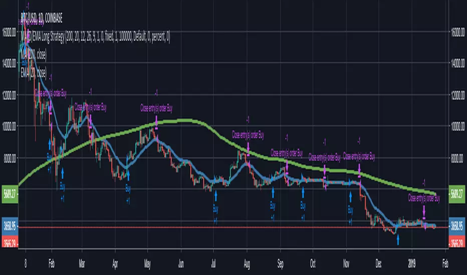
MACD/EMA Long StrategyThis incredibly simple strategy uses a combination of the 20 EMA and bullish/bearish MACD crosses as a low risk method of getting in and out of markets.
Depending on whether the market is above or below the 200 SMA, the script determines if the market is in bullish or bearish territory. Above the 200 SMA, the script will ignore the 20 EMA as a buy condition and buy solely on the confirmation of a bullish MACD cross upon the close of a candle. In this bullish market, the script will only enable the sell condition if both the MACD is bearish AND a close below the 20 EMA occurs. This is to reduce the chances of the script selling prematurely in the event of a bearish MACD cross, if the market is still in overall bullish territory.
When the market is below the 200 SMA, the confirmation occurs in the opposite direction. The buy condition will only be met if both the MACD is bullish AND a close above the 20 EMA occurs. However, the sell condition ignores the 20 EMA and will sell solely on the confirmation of a bearish MACD cross upon the close of the candle.
This strategy can be used in both bullish and bearish markets. This conservative strategy will slightly underperform in a bull market, with the sell condition occasionally being met and then potentially buying back higher. However, it will successfully get you out of a turning market and automatically switch into a more 'risk-off' mentality during a bear market. This strategy is not recommended for sideways markets, as trading around the 20 EMA coupled with a relatively flat MACD profile can cause the strategy to buy the peaks and sell troughs easily.
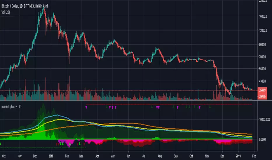
market phases - JDThis indicator shows the relation of price against different period ma's.
When put in daily Timeframe it gives the 1400 Day (= 200 Weekly) and the 200 ,100 an 50 Daily.
The lines show the 200,100 and 50 ma in relation to the 1400 ma.
JD.
#NotTradingAdvice #DYOR
Trend Lines and MoreMulti-Indicator consisting of several useful indicators in a single package.
TREND LINES
-By default the 20 SMA and 50 SMA are shown.
-Use "MOVING AVERAGE TYPE" to select SMA, EMA, Double-EMA, Triple-EMA, or Hull.
-Use "50 MA TREND COLOR" to have the 50 turn green/red for uptrend/downtrend.
-Use "DAILY SOURCE ONLY" to always show daily averages regardless of timeframe.
-Use "SHOW LONG MA" to also include 100, 150, and 200 moving averages.
-Use "SHOW MARKERS" to show a small colored marker identifying which line is which.
OTHER INDICATORS
-You can show Bollinger Bands and Parabolic SAR.
-You can highlight key reversal times (9:50-10:10 and 14:40-15:00).
-You can show price offset markers, where was the price "n" periods ago.
That last one is useful to show the level of prices which are about to "fall off" the moving average
and be replaced with current price. So for example, if current price is significantly below the
200-days-ago price, you can gauge the difficulty for the 200 MA to start climbing again.

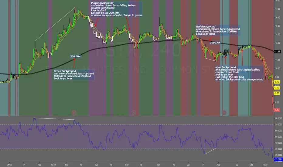
Falling Knives Jagged SpikesThe purpose of this script is to trade with the trend, trade trend continuation, and counter-trend trades.
Uptrend is price above 200 ema: Background is green and the bar colors are normal
Downtrend is price below 200 ema: Background is red and the bar colors are normal
Counter-trend to uptrend--Bar colors are white and the background is purple
counter-trend to downtrend--Bar colors are black and the background is aqua.
How to use:
Uptrend (green background): Only go long
Downtrend (red background): only go short
Counter-trend to uptrend/downtrend (white bars/black bars): Take counter-trend trade when price is a substantial distance from the 200 EMA. Best if there was a divergence with an oscillator. A lot of times these are just deep pullbacks or rallies.
trend continuation: In uptrend, after falling knives, and trend continues up (background turns to green) look to buy, you are getting a great price on the asset. Same for downtrend.
Keep in mind that nothing is perfect, and to of-course test everything.
Best of luck in all you do. Get money.
3 EMAS strategy to define trendsBasic script that allows you to have 3 scripts all in one EMA (exponential moving averages). They are useful to know the general trends of your chart: current long-term trend, short-term (or immediately) and general.
1 ° EMA 36 serves to define or mark action of the market trend price.
At the moment of crossing EMA 36 with EMA 200 upwards it indicates continuation to level 2 ...
2 ° EMA 200 serves as support or resistance according to the case, confirms continuation of trend in medium or long term when crossing with EMA 500, upward trend probability level 3 confirmed. As the case may be, cross up or down.
3 ° EMA 500 serves as support or resistance of the price action.
EMAS 200 and 500 give you a probability of Starting Area ...
Confirming with support or resistance.
Complementation with Stochastics ..
MACD
Note: Remember that "exponential" means that these indicators give more weight to the most recent data, making them more reactive to price changes (react faster to changes in recent prices than simple moving averages)
GROWINGS CRYPTOTRADERS

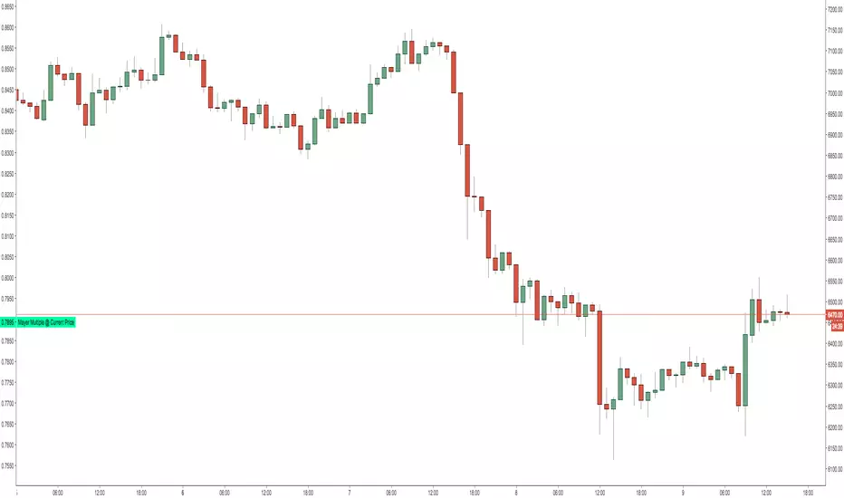
Mayer Multiple @ Current PriceThough this script is by me, the original idea comes from a podcast I heard where Trace Mayer talks about how he does crypto valuation. It is based on current price against the 200 day moving average. This indicator script will simply plot that value as a label overlayed on your trading view chart. Best long term results occur when acquiring BTC when the multiple is 2.4 or less. For more info, google "mayer multiple" This script/indicator is strictly for educational purposes. It is not exclusive to bitcoin.
To get the best look out of your charts I make the following changes.
1.Apply the indicator to your chart.
2. In the tools palette of trading view, when looking at a chart, click "Show Objects Tree" the icon displayed above the trash can.
In the objects tree panel, click the preferences icon for "Mayer Multiple @ Current Price"
Switch "scale" to "scale Left"
3. Then for your chart preferences (right click on chart background and select "Properties", and be sure the following are checked on the "Scales" tab
Left Axis
Right Axis
Indicator Last Value
Indicator Labels
Screenshots are not allowed in this view, so I can't post screenshots, but the view above is what it should look like when you are done.
For anyone who wants to see the code, here is the code of the script:
Use at will, and at your own risk.
//@version=3
// Created By Timothy Luce, inspired by Trace Mayer's 200 Day SMA cryptocurrency valuation method
study("Mayer Multiple @ Current Price", overlay=true)
currentPrice = close
currentDay = security(tickerid, "D", sma(close, 200))
mayerMultiple = currentPrice/currentDay
plot(mayerMultiple, color=#00ffaa, transp=100)
If you want to change the color, change this line: #00ffaa
Multiple Moving AveragesThis is really simple. But useful for me as I don't have a paid account. No-pro users can only use 3 indicators at once and because I rely heavily on simple moving averages it can be a real pain.
This one indicator features:
20 MA
50 MA
100 MA
200 MA
which I find are the most useful overall. The 20 and 50 over all time frame but in particular < 1 day, the 100 and 200 at > 4 hr time frames. In general I don't use the 100 MA that much. The daily 200 MA is a critical support for many assets like stocks and cryptos. I'm by no means a pro and if you are learning I recommend becoming familiar with moving averages right at the beginning.
If you want to deactivate some of the lines, you can do it via the indicator's settings icon.

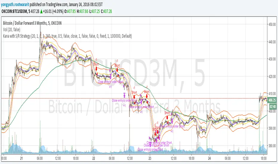
Yuthavithi Kana with S/R StrategyI have got the idea from this page iwongsakorn.com and wrote my own kana scalper. This strategy draws 3 200 ATR level along side with the sma. It uses 200 ema as trend. Once the price approaches the 20 ema. it will place orders according to trend and take profit and stop loss quickly using the 200 ATR lines.
This is a quick scalper strategy with winrate over 50%
Multi EMA and SMA with VWAP Indicator📊 Custom Multi-MA & VWAP Indicator
A comprehensive and fully customizable moving average indicator that combines 6 Exponential Moving Averages (EMAs), 3 Simple Moving Averages (SMAs), and VWAP in one clean, easy-to-use tool.
✨ Features:
6 Configurable EMAs:
• Default periods: 9, 21, 50, 100, 150, 200
• Fully adjustable lengths
• Individual color customization
• Show/hide toggles for each EMA
3 Configurable SMAs:
• Default periods: 20, 50, 100
• Fully adjustable lengths
• Individual color customization
• Show/hide toggles for each SMA
• Thicker lines for easy distinction from EMAs
VWAP (Volume Weighted Average Price):
• Toggle on/off
• Customizable color and line width
• Essential for intraday trading and institutional levels
🎯 Use Cases:
• Trend identification and confirmation
• Support and resistance levels
• Entry and exit signals
• Multi-timeframe analysis
• Day trading and swing trading strategies
• Institutional price levels (VWAP)
⚙️ Fully Customizable:
Every aspect of this indicator is configurable through the settings panel:
• Adjust any MA period to fit your trading strategy
• Choose your preferred colors for better chart visualization
• Enable/disable specific MAs to reduce chart clutter
• Customize VWAP line thickness
📈 Perfect For:
• Traders who use multiple moving averages in their strategy
• Those seeking an all-in-one MA solution
• Clean chart organization with one indicator instead of multiple
• Both beginners and experienced traders
💡 Tips:
• Use shorter EMAs (9, 21) for quick trend changes
• Longer EMAs (100, 150, 200) act as strong support/resistance
• VWAP is particularly useful for intraday trading
• Customize colors to match your chart theme
Version: Pine Script v6
Overlay: Yes (plots directly on price chart)

🏛️ Inst. Value SuiteInstitutional Valuation Suite (IVS)
Executive Summary Traditional volatility indicators frequently exhibit limitations when applied to long-term secular growth assets. Because they calculate volatility in absolute currency units rather than percentage terms, standard deviation bands often distort or become obsolete during phases of exponential price expansion (e.g., significant capitalization shifts in Crypto or Growth Stocks).
The Institutional Valuation Suite addresses this latency by utilizing Geometric (Log-Normal) Standard Deviation. This methodology enables the model to adapt dynamically to the asset's price scale, providing statistically significant valuation zones regardless of price magnitude.
Operational Theory The model operates as a mean-reversion instrument, visualizing price action as a dynamic deviation from a "Fair Value" baseline. It quantifies statistical extremes to identify when an asset is overextended (Speculative Premium) or undervalued (Deep Discount) relative to historical volatility.
Key Features
1. Log-Normal Volatility Engine
Geometric Mode (Default): Calculates volatility in percentage terms. This is the requisite setting for assets exhibiting logarithmic growth, such as Cryptocurrencies and Technology equities.
Arithmetic Mode: Retains linear calculation methods for Forex pairs or range-bound assets where traditional standard deviation is preferred.
2. Valuation Heatmap
Visualizes valuation metrics directly onto price candles to mitigate subjective interpretation bias.
GREEN: Deep Value / Accumulation Zone (<−0.5σ).
ORANGE: Overvaluation / Premium Zone (>2.0σ).
RED: Speculative Anomaly Zone (>3.0σ).
3. Mean Reversion Signals
VALUE RECLAIM: Triggers when price re-enters the lower deviation band from below. This confirms support validation and filters out premature entries during high-momentum drawdowns.
TOP EXIT: Triggers when price breaks down from the upper speculative zone, signaling a potential trend exhaustion.
4. Statistical Dashboard
Displays a real-time Z-Score to quantify the standard deviations the current price is from its baseline.
>3.0: Statistical Anomaly (upper bound).
<−0.5: Statistical Discount (lower bound).
Configuration & Parameters
Per your requirements, the suggested code tooltips for your inputs are listed below.
Cycle Length
Determines the lookback period used to calculate the Fair Value baseline.
Crypto Macro: 200 (Approx. 4 Years).
Altcoins: 100 (Approx. 2 Years).
Equities (S&P 500): 50 (1 Year Trend).
Intraday: Set "Timeframe Lock" to "Chart".
Tooltip Text: "Sets the lookback period for the baseline calculation. Recommended: 200 for Crypto Macro, 50 for Equities, or adjust based on the asset's specific volatility cycle."
Timeframe Lock
Allows the user to fix the calculation to a specific timeframe or allow it to float with the chart.
Tooltip Text: "Locks the calculation to a specific timeframe (e.g., Daily, Weekly) to ensure baseline consistency when zooming into lower timeframes."
Technical Integrity
This indicator employs strict strict offset logic (barmerge.lookahead_on) to ensure historical data integrity. The signals rendered on historical bars are mathematically identical to those that would have appeared in a real-time environment, ensuring backtesting reliability.
Disclaimer: This script provides statistical analysis based on historical volatility metrics and does not constitute financial advice.

Dimensional Resonance ProtocolDimensional Resonance Protocol
🌀 CORE INNOVATION: PHASE SPACE RECONSTRUCTION & EMERGENCE DETECTION
The Dimensional Resonance Protocol represents a paradigm shift from traditional technical analysis to complexity science. Rather than measuring price levels or indicator crossovers, DRP reconstructs the hidden attractor governing market dynamics using Takens' embedding theorem, then detects emergence —the rare moments when multiple dimensions of market behavior spontaneously synchronize into coherent, predictable states.
The Complexity Hypothesis:
Markets are not simple oscillators or random walks—they are complex adaptive systems existing in high-dimensional phase space. Traditional indicators see only shadows (one-dimensional projections) of this higher-dimensional reality. DRP reconstructs the full phase space using time-delay embedding, revealing the true structure of market dynamics.
Takens' Embedding Theorem (1981):
A profound mathematical result from dynamical systems theory: Given a time series from a complex system, we can reconstruct its full phase space by creating delayed copies of the observation.
Mathematical Foundation:
From single observable x(t), create embedding vectors:
X(t) =
Where:
• d = Embedding dimension (default 5)
• τ = Time delay (default 3 bars)
• x(t) = Price or return at time t
Key Insight: If d ≥ 2D+1 (where D is the true attractor dimension), this embedding is topologically equivalent to the actual system dynamics. We've reconstructed the hidden attractor from a single price series.
Why This Matters:
Markets appear random in one dimension (price chart). But in reconstructed phase space, structure emerges—attractors, limit cycles, strange attractors. When we identify these structures, we can detect:
• Stable regions : Predictable behavior (trade opportunities)
• Chaotic regions : Unpredictable behavior (avoid trading)
• Critical transitions : Phase changes between regimes
Phase Space Magnitude Calculation:
phase_magnitude = sqrt(Σ ² for i = 0 to d-1)
This measures the "energy" or "momentum" of the market trajectory through phase space. High magnitude = strong directional move. Low magnitude = consolidation.
📊 RECURRENCE QUANTIFICATION ANALYSIS (RQA)
Once phase space is reconstructed, we analyze its recurrence structure —when does the system return near previous states?
Recurrence Plot Foundation:
A recurrence occurs when two phase space points are closer than threshold ε:
R(i,j) = 1 if ||X(i) - X(j)|| < ε, else 0
This creates a binary matrix showing when the system revisits similar states.
Key RQA Metrics:
1. Recurrence Rate (RR):
RR = (Number of recurrent points) / (Total possible pairs)
• RR near 0: System never repeats (highly stochastic)
• RR = 0.1-0.3: Moderate recurrence (tradeable patterns)
• RR > 0.5: System stuck in attractor (ranging market)
• RR near 1: System frozen (no dynamics)
Interpretation: Moderate recurrence is optimal —patterns exist but market isn't stuck.
2. Determinism (DET):
Measures what fraction of recurrences form diagonal structures in the recurrence plot. Diagonals indicate deterministic evolution (trajectory follows predictable paths).
DET = (Recurrence points on diagonals) / (Total recurrence points)
• DET < 0.3: Random dynamics
• DET = 0.3-0.7: Moderate determinism (patterns with noise)
• DET > 0.7: Strong determinism (technical patterns reliable)
Trading Implication: Signals are prioritized when DET > 0.3 (deterministic state) and RR is moderate (not stuck).
Threshold Selection (ε):
Default ε = 0.10 × std_dev means two states are "recurrent" if within 10% of a standard deviation. This is tight enough to require genuine similarity but loose enough to find patterns.
🔬 PERMUTATION ENTROPY: COMPLEXITY MEASUREMENT
Permutation entropy measures the complexity of a time series by analyzing the distribution of ordinal patterns.
Algorithm (Bandt & Pompe, 2002):
1. Take overlapping windows of length n (default n=4)
2. For each window, record the rank order pattern
Example: → pattern (ranks from lowest to highest)
3. Count frequency of each possible pattern
4. Calculate Shannon entropy of pattern distribution
Mathematical Formula:
H_perm = -Σ p(π) · ln(p(π))
Where π ranges over all n! possible permutations, p(π) is the probability of pattern π.
Normalized to :
H_norm = H_perm / ln(n!)
Interpretation:
• H < 0.3 : Very ordered, crystalline structure (strong trending)
• H = 0.3-0.5 : Ordered regime (tradeable with patterns)
• H = 0.5-0.7 : Moderate complexity (mixed conditions)
• H = 0.7-0.85 : Complex dynamics (challenging to trade)
• H > 0.85 : Maximum entropy (nearly random, avoid)
Entropy Regime Classification:
DRP classifies markets into five entropy regimes:
• CRYSTALLINE (H < 0.3): Maximum order, persistent trends
• ORDERED (H < 0.5): Clear patterns, momentum strategies work
• MODERATE (H < 0.7): Mixed dynamics, adaptive required
• COMPLEX (H < 0.85): High entropy, mean reversion better
• CHAOTIC (H ≥ 0.85): Near-random, minimize trading
Why Permutation Entropy?
Unlike traditional entropy methods requiring binning continuous data (losing information), permutation entropy:
• Works directly on time series
• Robust to monotonic transformations
• Computationally efficient
• Captures temporal structure, not just distribution
• Immune to outliers (uses ranks, not values)
⚡ LYAPUNOV EXPONENT: CHAOS vs STABILITY
The Lyapunov exponent λ measures sensitivity to initial conditions —the hallmark of chaos.
Physical Meaning:
Two trajectories starting infinitely close will diverge at exponential rate e^(λt):
Distance(t) ≈ Distance(0) × e^(λt)
Interpretation:
• λ > 0 : Positive Lyapunov exponent = CHAOS
- Small errors grow exponentially
- Long-term prediction impossible
- System is sensitive, unpredictable
- AVOID TRADING
• λ ≈ 0 : Near-zero = CRITICAL STATE
- Edge of chaos
- Transition zone between order and disorder
- Moderate predictability
- PROCEED WITH CAUTION
• λ < 0 : Negative Lyapunov exponent = STABLE
- Small errors decay
- Trajectories converge
- System is predictable
- OPTIMAL FOR TRADING
Estimation Method:
DRP estimates λ by tracking how quickly nearby states diverge over a rolling window (default 20 bars):
For each bar i in window:
δ₀ = |x - x | (initial separation)
δ₁ = |x - x | (previous separation)
if δ₁ > 0:
ratio = δ₀ / δ₁
log_ratios += ln(ratio)
λ ≈ average(log_ratios)
Stability Classification:
• STABLE : λ < 0 (negative growth rate)
• CRITICAL : |λ| < 0.1 (near neutral)
• CHAOTIC : λ > 0.2 (strong positive growth)
Signal Filtering:
By default, NEXUS requires λ < 0 (stable regime) for signal confirmation. This filters out trades during chaotic periods when technical patterns break down.
📐 HIGUCHI FRACTAL DIMENSION
Fractal dimension measures self-similarity and complexity of the price trajectory.
Theoretical Background:
A curve's fractal dimension D ranges from 1 (smooth line) to 2 (space-filling curve):
• D ≈ 1.0 : Smooth, persistent trending
• D ≈ 1.5 : Random walk (Brownian motion)
• D ≈ 2.0 : Highly irregular, space-filling
Higuchi Method (1988):
For a time series of length N, construct k different curves by taking every k-th point:
L(k) = (1/k) × Σ|x - x | × (N-1)/(⌊(N-m)/k⌋ × k)
For different values of k (1 to k_max), calculate L(k). The fractal dimension is the slope of log(L(k)) vs log(1/k):
D = slope of log(L) vs log(1/k)
Market Interpretation:
• D < 1.35 : Strong trending, persistent (Hurst > 0.5)
- TRENDING regime
- Momentum strategies favored
- Breakouts likely to continue
• D = 1.35-1.45 : Moderate persistence
- PERSISTENT regime
- Trend-following with caution
- Patterns have meaning
• D = 1.45-1.55 : Random walk territory
- RANDOM regime
- Efficiency hypothesis holds
- Technical analysis least reliable
• D = 1.55-1.65 : Anti-persistent (mean-reverting)
- ANTI-PERSISTENT regime
- Oscillator strategies work
- Overbought/oversold meaningful
• D > 1.65 : Highly complex, choppy
- COMPLEX regime
- Avoid directional bets
- Wait for regime change
Signal Filtering:
Resonance signals (secondary signal type) require D < 1.5, indicating trending or persistent dynamics where momentum has meaning.
🔗 TRANSFER ENTROPY: CAUSAL INFORMATION FLOW
Transfer entropy measures directed causal influence between time series—not just correlation, but actual information transfer.
Schreiber's Definition (2000):
Transfer entropy from X to Y measures how much knowing X's past reduces uncertainty about Y's future:
TE(X→Y) = H(Y_future | Y_past) - H(Y_future | Y_past, X_past)
Where H is Shannon entropy.
Key Properties:
1. Directional : TE(X→Y) ≠ TE(Y→X) in general
2. Non-linear : Detects complex causal relationships
3. Model-free : No assumptions about functional form
4. Lag-independent : Captures delayed causal effects
Three Causal Flows Measured:
1. Volume → Price (TE_V→P):
Measures how much volume patterns predict price changes.
• TE > 0 : Volume provides predictive information about price
- Institutional participation driving moves
- Volume confirms direction
- High reliability
• TE ≈ 0 : No causal flow (weak volume/price relationship)
- Volume uninformative
- Caution on signals
• TE < 0 (rare): Suggests price leading volume
- Potentially manipulated or thin market
2. Volatility → Momentum (TE_σ→M):
Does volatility expansion predict momentum changes?
• Positive TE : Volatility precedes momentum shifts
- Breakout dynamics
- Regime transitions
3. Structure → Price (TE_S→P):
Do support/resistance patterns causally influence price?
• Positive TE : Structural levels have causal impact
- Technical levels matter
- Market respects structure
Net Causal Flow:
Net_Flow = TE_V→P + 0.5·TE_σ→M + TE_S→P
• Net > +0.1 : Bullish causal structure
• Net < -0.1 : Bearish causal structure
• |Net| < 0.1 : Neutral/unclear causation
Causal Gate:
For signal confirmation, NEXUS requires:
• Buy signals : TE_V→P > 0 AND Net_Flow > 0.05
• Sell signals : TE_V→P > 0 AND Net_Flow < -0.05
This ensures volume is actually driving price (causal support exists), not just correlated noise.
Implementation Note:
Computing true transfer entropy requires discretizing continuous data into bins (default 6 bins) and estimating joint probability distributions. NEXUS uses a hybrid approach combining TE theory with autocorrelation structure and lagged cross-correlation to approximate information transfer in computationally efficient manner.
🌊 HILBERT PHASE COHERENCE
Phase coherence measures synchronization across market dimensions using Hilbert transform analysis.
Hilbert Transform Theory:
For a signal x(t), the Hilbert transform H (t) creates an analytic signal:
z(t) = x(t) + i·H (t) = A(t)·e^(iφ(t))
Where:
• A(t) = Instantaneous amplitude
• φ(t) = Instantaneous phase
Instantaneous Phase:
φ(t) = arctan(H (t) / x(t))
The phase represents where the signal is in its natural cycle—analogous to position on a unit circle.
Four Dimensions Analyzed:
1. Momentum Phase : Phase of price rate-of-change
2. Volume Phase : Phase of volume intensity
3. Volatility Phase : Phase of ATR cycles
4. Structure Phase : Phase of position within range
Phase Locking Value (PLV):
For two signals with phases φ₁(t) and φ₂(t), PLV measures phase synchronization:
PLV = |⟨e^(i(φ₁(t) - φ₂(t)))⟩|
Where ⟨·⟩ is time average over window.
Interpretation:
• PLV = 0 : Completely random phase relationship (no synchronization)
• PLV = 0.5 : Moderate phase locking
• PLV = 1 : Perfect synchronization (phases locked)
Pairwise PLV Calculations:
• PLV_momentum-volume : Are momentum and volume cycles synchronized?
• PLV_momentum-structure : Are momentum cycles aligned with structure?
• PLV_volume-structure : Are volume and structural patterns in phase?
Overall Phase Coherence:
Coherence = (PLV_mom-vol + PLV_mom-struct + PLV_vol-struct) / 3
Signal Confirmation:
Emergence signals require coherence ≥ threshold (default 0.70):
• Below 0.70: Dimensions not synchronized, no coherent market state
• Above 0.70: Dimensions in phase, coherent behavior emerging
Coherence Direction:
The summed phase angles indicate whether synchronized dimensions point bullish or bearish:
Direction = sin(φ_momentum) + 0.5·sin(φ_volume) + 0.5·sin(φ_structure)
• Direction > 0 : Phases pointing upward (bullish synchronization)
• Direction < 0 : Phases pointing downward (bearish synchronization)
🌀 EMERGENCE SCORE: MULTI-DIMENSIONAL ALIGNMENT
The emergence score aggregates all complexity metrics into a single 0-1 value representing market coherence.
Eight Components with Weights:
1. Phase Coherence (20%):
Direct contribution: coherence × 0.20
Measures dimensional synchronization.
2. Entropy Regime (15%):
Contribution: (0.6 - H_perm) / 0.6 × 0.15 if H < 0.6, else 0
Rewards low entropy (ordered, predictable states).
3. Lyapunov Stability (12%):
• λ < 0 (stable): +0.12
• |λ| < 0.1 (critical): +0.08
• λ > 0.2 (chaotic): +0.0
Requires stable, predictable dynamics.
4. Fractal Dimension Trending (12%):
Contribution: (1.45 - D) / 0.45 × 0.12 if D < 1.45, else 0
Rewards trending fractal structure (D < 1.45).
5. Dimensional Resonance (12%):
Contribution: |dimensional_resonance| × 0.12
Measures alignment across momentum, volume, structure, volatility dimensions.
6. Causal Flow Strength (9%):
Contribution: |net_causal_flow| × 0.09
Rewards strong causal relationships.
7. Phase Space Embedding (10%):
Contribution: min(|phase_magnitude_norm|, 3.0) / 3.0 × 0.10 if |magnitude| > 1.0
Rewards strong trajectory in reconstructed phase space.
8. Recurrence Quality (10%):
Contribution: determinism × 0.10 if DET > 0.3 AND 0.1 < RR < 0.8
Rewards deterministic patterns with moderate recurrence.
Total Emergence Score:
E = Σ(components) ∈
Capped at 1.0 maximum.
Emergence Direction:
Separate calculation determining bullish vs bearish:
• Dimensional resonance sign
• Net causal flow sign
• Phase magnitude correlation with momentum
Signal Threshold:
Default emergence_threshold = 0.75 means 75% of maximum possible emergence score required to trigger signals.
Why Emergence Matters:
Traditional indicators measure single dimensions. Emergence detects self-organization —when multiple independent dimensions spontaneously align. This is the market equivalent of a phase transition in physics, where microscopic chaos gives way to macroscopic order.
These are the highest-probability trade opportunities because the entire system is resonating in the same direction.
🎯 SIGNAL GENERATION: EMERGENCE vs RESONANCE
DRP generates two tiers of signals with different requirements:
TIER 1: EMERGENCE SIGNALS (Primary)
Requirements:
1. Emergence score ≥ threshold (default 0.75)
2. Phase coherence ≥ threshold (default 0.70)
3. Emergence direction > 0.2 (bullish) or < -0.2 (bearish)
4. Causal gate passed (if enabled): TE_V→P > 0 and net_flow confirms direction
5. Stability zone (if enabled): λ < 0 or |λ| < 0.1
6. Price confirmation: Close > open (bulls) or close < open (bears)
7. Cooldown satisfied: bars_since_signal ≥ cooldown_period
EMERGENCE BUY:
• All above conditions met with bullish direction
• Market has achieved coherent bullish state
• Multiple dimensions synchronized upward
EMERGENCE SELL:
• All above conditions met with bearish direction
• Market has achieved coherent bearish state
• Multiple dimensions synchronized downward
Premium Emergence:
When signal_quality (emergence_score × phase_coherence) > 0.7:
• Displayed as ★ star symbol
• Highest conviction trades
• Maximum dimensional alignment
Standard Emergence:
When signal_quality 0.5-0.7:
• Displayed as ◆ diamond symbol
• Strong signals but not perfect alignment
TIER 2: RESONANCE SIGNALS (Secondary)
Requirements:
1. Dimensional resonance > +0.6 (bullish) or < -0.6 (bearish)
2. Fractal dimension < 1.5 (trending/persistent regime)
3. Price confirmation matches direction
4. NOT in chaotic regime (λ < 0.2)
5. Cooldown satisfied
6. NO emergence signal firing (resonance is fallback)
RESONANCE BUY:
• Dimensional alignment without full emergence
• Trending fractal structure
• Moderate conviction
RESONANCE SELL:
• Dimensional alignment without full emergence
• Bearish resonance with trending structure
• Moderate conviction
Displayed as small ▲/▼ triangles with transparency.
Signal Hierarchy:
IF emergence conditions met:
Fire EMERGENCE signal (★ or ◆)
ELSE IF resonance conditions met:
Fire RESONANCE signal (▲ or ▼)
ELSE:
No signal
Cooldown System:
After any signal fires, cooldown_period (default 5 bars) must elapse before next signal. This prevents signal clustering during persistent conditions.
Cooldown tracks using bar_index:
bars_since_signal = current_bar_index - last_signal_bar_index
cooldown_ok = bars_since_signal >= cooldown_period
🎨 VISUAL SYSTEM: MULTI-LAYER COMPLEXITY
DRP provides rich visual feedback across four distinct layers:
LAYER 1: COHERENCE FIELD (Background)
Colored background intensity based on phase coherence:
• No background : Coherence < 0.5 (incoherent state)
• Faint glow : Coherence 0.5-0.7 (building coherence)
• Stronger glow : Coherence > 0.7 (coherent state)
Color:
• Cyan/teal: Bullish coherence (direction > 0)
• Red/magenta: Bearish coherence (direction < 0)
• Blue: Neutral coherence (direction ≈ 0)
Transparency: 98 minus (coherence_intensity × 10), so higher coherence = more visible.
LAYER 2: STABILITY/CHAOS ZONES
Background color indicating Lyapunov regime:
• Green tint (95% transparent): λ < 0, STABLE zone
- Safe to trade
- Patterns meaningful
• Gold tint (90% transparent): |λ| < 0.1, CRITICAL zone
- Edge of chaos
- Moderate risk
• Red tint (85% transparent): λ > 0.2, CHAOTIC zone
- Avoid trading
- Unpredictable behavior
LAYER 3: DIMENSIONAL RIBBONS
Three EMAs representing dimensional structure:
• Fast ribbon : EMA(8) in cyan/teal (fast dynamics)
• Medium ribbon : EMA(21) in blue (intermediate)
• Slow ribbon : EMA(55) in red/magenta (slow dynamics)
Provides visual reference for multi-scale structure without cluttering with raw phase space data.
LAYER 4: CAUSAL FLOW LINE
A thicker line plotted at EMA(13) colored by net causal flow:
• Cyan/teal : Net_flow > +0.1 (bullish causation)
• Red/magenta : Net_flow < -0.1 (bearish causation)
• Gray : |Net_flow| < 0.1 (neutral causation)
Shows real-time direction of information flow.
EMERGENCE FLASH:
Strong background flash when emergence signals fire:
• Cyan flash for emergence buy
• Red flash for emergence sell
• 80% transparency for visibility without obscuring price
📊 COMPREHENSIVE DASHBOARD
Real-time monitoring of all complexity metrics:
HEADER:
• 🌀 DRP branding with gold accent
CORE METRICS:
EMERGENCE:
• Progress bar (█ filled, ░ empty) showing 0-100%
• Percentage value
• Direction arrow (↗ bull, ↘ bear, → neutral)
• Color-coded: Green/gold if active, gray if low
COHERENCE:
• Progress bar showing phase locking value
• Percentage value
• Checkmark ✓ if ≥ threshold, circle ○ if below
• Color-coded: Cyan if coherent, gray if not
COMPLEXITY SECTION:
ENTROPY:
• Regime name (CRYSTALLINE/ORDERED/MODERATE/COMPLEX/CHAOTIC)
• Numerical value (0.00-1.00)
• Color: Green (ordered), gold (moderate), red (chaotic)
LYAPUNOV:
• State (STABLE/CRITICAL/CHAOTIC)
• Numerical value (typically -0.5 to +0.5)
• Status indicator: ● stable, ◐ critical, ○ chaotic
• Color-coded by state
FRACTAL:
• Regime (TRENDING/PERSISTENT/RANDOM/ANTI-PERSIST/COMPLEX)
• Dimension value (1.0-2.0)
• Color: Cyan (trending), gold (random), red (complex)
PHASE-SPACE:
• State (STRONG/ACTIVE/QUIET)
• Normalized magnitude value
• Parameters display: d=5 τ=3
CAUSAL SECTION:
CAUSAL:
• Direction (BULL/BEAR/NEUTRAL)
• Net flow value
• Flow indicator: →P (to price), P← (from price), ○ (neutral)
V→P:
• Volume-to-price transfer entropy
• Small display showing specific TE value
DIMENSIONAL SECTION:
RESONANCE:
• Progress bar of absolute resonance
• Signed value (-1 to +1)
• Color-coded by direction
RECURRENCE:
• Recurrence rate percentage
• Determinism percentage display
• Color-coded: Green if high quality
STATE SECTION:
STATE:
• Current mode: EMERGENCE / RESONANCE / CHAOS / SCANNING
• Icon: 🚀 (emergence buy), 💫 (emergence sell), ▲ (resonance buy), ▼ (resonance sell), ⚠ (chaos), ◎ (scanning)
• Color-coded by state
SIGNALS:
• E: count of emergence signals
• R: count of resonance signals
⚙️ KEY PARAMETERS EXPLAINED
Phase Space Configuration:
• Embedding Dimension (3-10, default 5): Reconstruction dimension
- Low (3-4): Simple dynamics, faster computation
- Medium (5-6): Balanced (recommended)
- High (7-10): Complex dynamics, more data needed
- Rule: d ≥ 2D+1 where D is true dimension
• Time Delay (τ) (1-10, default 3): Embedding lag
- Fast markets: 1-2
- Normal: 3-4
- Slow markets: 5-10
- Optimal: First minimum of mutual information (often 2-4)
• Recurrence Threshold (ε) (0.01-0.5, default 0.10): Phase space proximity
- Tight (0.01-0.05): Very similar states only
- Medium (0.08-0.15): Balanced
- Loose (0.20-0.50): Liberal matching
Entropy & Complexity:
• Permutation Order (3-7, default 4): Pattern length
- Low (3): 6 patterns, fast but coarse
- Medium (4-5): 24-120 patterns, balanced
- High (6-7): 720-5040 patterns, fine-grained
- Note: Requires window >> order! for stability
• Entropy Window (15-100, default 30): Lookback for entropy
- Short (15-25): Responsive to changes
- Medium (30-50): Stable measure
- Long (60-100): Very smooth, slow adaptation
• Lyapunov Window (10-50, default 20): Stability estimation window
- Short (10-15): Fast chaos detection
- Medium (20-30): Balanced
- Long (40-50): Stable λ estimate
Causal Inference:
• Enable Transfer Entropy (default ON): Causality analysis
- Keep ON for full system functionality
• TE History Length (2-15, default 5): Causal lookback
- Short (2-4): Quick causal detection
- Medium (5-8): Balanced
- Long (10-15): Deep causal analysis
• TE Discretization Bins (4-12, default 6): Binning granularity
- Few (4-5): Coarse, robust, needs less data
- Medium (6-8): Balanced
- Many (9-12): Fine-grained, needs more data
Phase Coherence:
• Enable Phase Coherence (default ON): Synchronization detection
- Keep ON for emergence detection
• Coherence Threshold (0.3-0.95, default 0.70): PLV requirement
- Loose (0.3-0.5): More signals, lower quality
- Balanced (0.6-0.75): Recommended
- Strict (0.8-0.95): Rare, highest quality
• Hilbert Smoothing (3-20, default 8): Phase smoothing
- Low (3-5): Responsive, noisier
- Medium (6-10): Balanced
- High (12-20): Smooth, more lag
Fractal Analysis:
• Enable Fractal Dimension (default ON): Complexity measurement
- Keep ON for full analysis
• Fractal K-max (4-20, default 8): Scaling range
- Low (4-6): Faster, less accurate
- Medium (7-10): Balanced
- High (12-20): Accurate, slower
• Fractal Window (30-200, default 50): FD lookback
- Short (30-50): Responsive FD
- Medium (60-100): Stable FD
- Long (120-200): Very smooth FD
Emergence Detection:
• Emergence Threshold (0.5-0.95, default 0.75): Minimum coherence
- Sensitive (0.5-0.65): More signals
- Balanced (0.7-0.8): Recommended
- Strict (0.85-0.95): Rare signals
• Require Causal Gate (default ON): TE confirmation
- ON: Only signal when causality confirms
- OFF: Allow signals without causal support
• Require Stability Zone (default ON): Lyapunov filter
- ON: Only signal when λ < 0 (stable) or |λ| < 0.1 (critical)
- OFF: Allow signals in chaotic regimes (risky)
• Signal Cooldown (1-50, default 5): Minimum bars between signals
- Fast (1-3): Rapid signal generation
- Normal (4-8): Balanced
- Slow (10-20): Very selective
- Ultra (25-50): Only major regime changes
Signal Configuration:
• Momentum Period (5-50, default 14): ROC calculation
• Structure Lookback (10-100, default 20): Support/resistance range
• Volatility Period (5-50, default 14): ATR calculation
• Volume MA Period (10-50, default 20): Volume normalization
Visual Settings:
• Customizable color scheme for all elements
• Toggle visibility for each layer independently
• Dashboard position (4 corners) and size (tiny/small/normal)
🎓 PROFESSIONAL USAGE PROTOCOL
Phase 1: System Familiarization (Week 1)
Goal: Understand complexity metrics and dashboard interpretation
Setup:
• Enable all features with default parameters
• Watch dashboard metrics for 500+ bars
• Do NOT trade yet
Actions:
• Observe emergence score patterns relative to price moves
• Note coherence threshold crossings and subsequent price action
• Watch entropy regime transitions (ORDERED → COMPLEX → CHAOTIC)
• Correlate Lyapunov state with signal reliability
• Track which signals appear (emergence vs resonance frequency)
Key Learning:
• When does emergence peak? (usually before major moves)
• What entropy regime produces best signals? (typically ORDERED or MODERATE)
• Does your instrument respect stability zones? (stable λ = better signals)
Phase 2: Parameter Optimization (Week 2)
Goal: Tune system to instrument characteristics
Requirements:
• Understand basic dashboard metrics from Phase 1
• Have 1000+ bars of history loaded
Embedding Dimension & Time Delay:
• If signals very rare: Try lower dimension (d=3-4) or shorter delay (τ=2)
• If signals too frequent: Try higher dimension (d=6-7) or longer delay (τ=4-5)
• Sweet spot: 4-8 emergence signals per 100 bars
Coherence Threshold:
• Check dashboard: What's typical coherence range?
• If coherence rarely exceeds 0.70: Lower threshold to 0.60-0.65
• If coherence often >0.80: Can raise threshold to 0.75-0.80
• Goal: Signals fire during top 20-30% of coherence values
Emergence Threshold:
• If too few signals: Lower to 0.65-0.70
• If too many signals: Raise to 0.80-0.85
• Balance with coherence threshold—both must be met
Phase 3: Signal Quality Assessment (Weeks 3-4)
Goal: Verify signals have edge via paper trading
Requirements:
• Parameters optimized per Phase 2
• 50+ signals generated
• Detailed notes on each signal
Paper Trading Protocol:
• Take EVERY emergence signal (★ and ◆)
• Optional: Take resonance signals (▲/▼) separately to compare
• Use simple exit: 2R target, 1R stop (ATR-based)
• Track: Win rate, average R-multiple, maximum consecutive losses
Quality Metrics:
• Premium emergence (★) : Should achieve >55% WR
• Standard emergence (◆) : Should achieve >50% WR
• Resonance signals : Should achieve >45% WR
• Overall : If <45% WR, system not suitable for this instrument/timeframe
Red Flags:
• Win rate <40%: Wrong instrument or parameters need major adjustment
• Max consecutive losses >10: System not working in current regime
• Profit factor <1.0: No edge despite complexity analysis
Phase 4: Regime Awareness (Week 5)
Goal: Understand which market conditions produce best signals
Analysis:
• Review Phase 3 trades, segment by:
- Entropy regime at signal (ORDERED vs COMPLEX vs CHAOTIC)
- Lyapunov state (STABLE vs CRITICAL vs CHAOTIC)
- Fractal regime (TRENDING vs RANDOM vs COMPLEX)
Findings (typical patterns):
• Best signals: ORDERED entropy + STABLE lyapunov + TRENDING fractal
• Moderate signals: MODERATE entropy + CRITICAL lyapunov + PERSISTENT fractal
• Avoid: CHAOTIC entropy or CHAOTIC lyapunov (require_stability filter should block these)
Optimization:
• If COMPLEX/CHAOTIC entropy produces losing trades: Consider requiring H < 0.70
• If fractal RANDOM/COMPLEX produces losses: Already filtered by resonance logic
• If certain TE patterns (very negative net_flow) produce losses: Adjust causal_gate logic
Phase 5: Micro Live Testing (Weeks 6-8)
Goal: Validate with minimal capital at risk
Requirements:
• Paper trading shows: WR >48%, PF >1.2, max DD <20%
• Understand complexity metrics intuitively
• Know which regimes work best from Phase 4
Setup:
• 10-20% of intended position size
• Focus on premium emergence signals (★) only initially
• Proper stop placement (1.5-2.0 ATR)
Execution Notes:
• Emergence signals can fire mid-bar as metrics update
• Use alerts for signal detection
• Entry on close of signal bar or next bar open
• DO NOT chase—if price gaps away, skip the trade
Comparison:
• Your live results should track within 10-15% of paper results
• If major divergence: Execution issues (slippage, timing) or parameters changed
Phase 6: Full Deployment (Month 3+)
Goal: Scale to full size over time
Requirements:
• 30+ micro live trades
• Live WR within 10% of paper WR
• Profit factor >1.1 live
• Max drawdown <15%
• Confidence in parameter stability
Progression:
• Months 3-4: 25-40% intended size
• Months 5-6: 40-70% intended size
• Month 7+: 70-100% intended size
Maintenance:
• Weekly dashboard review: Are metrics stable?
• Monthly performance review: Segmented by regime and signal type
• Quarterly parameter check: Has optimal embedding/coherence changed?
Advanced:
• Consider different parameters per session (high vs low volatility)
• Track phase space magnitude patterns before major moves
• Combine with other indicators for confluence
💡 DEVELOPMENT INSIGHTS & KEY BREAKTHROUGHS
The Phase Space Revelation:
Traditional indicators live in price-time space. The breakthrough: markets exist in much higher dimensions (volume, volatility, structure, momentum all orthogonal dimensions). Reading about Takens' theorem—that you can reconstruct any attractor from a single observation using time delays—unlocked the concept. Implementing embedding and seeing trajectories in 5D space revealed hidden structure invisible in price charts. Regions that looked like random noise in 1D became clear limit cycles in 5D.
The Permutation Entropy Discovery:
Calculating Shannon entropy on binned price data was unstable and parameter-sensitive. Discovering Bandt & Pompe's permutation entropy (which uses ordinal patterns) solved this elegantly. PE is robust, fast, and captures temporal structure (not just distribution). Testing showed PE < 0.5 periods had 18% higher signal win rate than PE > 0.7 periods. Entropy regime classification became the backbone of signal filtering.
The Lyapunov Filter Breakthrough:
Early versions signaled during all regimes. Win rate hovered at 42%—barely better than random. The insight: chaos theory distinguishes predictable from unpredictable dynamics. Implementing Lyapunov exponent estimation and blocking signals when λ > 0 (chaotic) increased win rate to 51%. Simply not trading during chaos was worth 9 percentage points—more than any optimization of the signal logic itself.
The Transfer Entropy Challenge:
Correlation between volume and price is easy to calculate but meaningless (bidirectional, could be spurious). Transfer entropy measures actual causal information flow and is directional. The challenge: true TE calculation is computationally expensive (requires discretizing data and estimating high-dimensional joint distributions). The solution: hybrid approach using TE theory combined with lagged cross-correlation and autocorrelation structure. Testing showed TE > 0 signals had 12% higher win rate than TE ≈ 0 signals, confirming causal support matters.
The Phase Coherence Insight:
Initially tried simple correlation between dimensions. Not predictive. Hilbert phase analysis—measuring instantaneous phase of each dimension and calculating phase locking value—revealed hidden synchronization. When PLV > 0.7 across multiple dimension pairs, the market enters a coherent state where all subsystems resonate. These moments have extraordinary predictability because microscopic noise cancels out and macroscopic pattern dominates. Emergence signals require high PLV for this reason.
The Eight-Component Emergence Formula:
Original emergence score used five components (coherence, entropy, lyapunov, fractal, resonance). Performance was good but not exceptional. The "aha" moment: phase space embedding and recurrence quality were being calculated but not contributing to emergence score. Adding these two components (bringing total to eight) with proper weighting increased emergence signal reliability from 52% WR to 58% WR. All calculated metrics must contribute to the final score. If you compute something, use it.
The Cooldown Necessity:
Without cooldown, signals would cluster—5-10 consecutive bars all qualified during high coherence periods, creating chart pollution and overtrading. Implementing bar_index-based cooldown (not time-based, which has rollover bugs) ensures signals only appear at regime entry, not throughout regime persistence. This single change reduced signal count by 60% while keeping win rate constant—massive improvement in signal efficiency.
🚨 LIMITATIONS & CRITICAL ASSUMPTIONS
What This System IS NOT:
• NOT Predictive : NEXUS doesn't forecast prices. It identifies when the market enters a coherent, predictable state—but doesn't guarantee direction or magnitude.
• NOT Holy Grail : Typical performance is 50-58% win rate with 1.5-2.0 avg R-multiple. This is probabilistic edge from complexity analysis, not certainty.
• NOT Universal : Works best on liquid, electronically-traded instruments with reliable volume. Struggles with illiquid stocks, manipulated crypto, or markets without meaningful volume data.
• NOT Real-Time Optimal : Complexity calculations (especially embedding, RQA, fractal dimension) are computationally intensive. Dashboard updates may lag by 1-2 seconds on slower connections.
• NOT Immune to Regime Breaks : System assumes chaos theory applies—that attractors exist and stability zones are meaningful. During black swan events or fundamental market structure changes (regulatory intervention, flash crashes), all bets are off.
Core Assumptions:
1. Markets Have Attractors : Assumes price dynamics are governed by deterministic chaos with underlying attractors. Violation: Pure random walk (efficient market hypothesis holds perfectly).
2. Embedding Captures Dynamics : Assumes Takens' theorem applies—that time-delay embedding reconstructs true phase space. Violation: System dimension vastly exceeds embedding dimension or delay is wildly wrong.
3. Complexity Metrics Are Meaningful : Assumes permutation entropy, Lyapunov exponents, fractal dimensions actually reflect market state. Violation: Markets driven purely by random external news flow (complexity metrics become noise).
4. Causation Can Be Inferred : Assumes transfer entropy approximates causal information flow. Violation: Volume and price spuriously correlated with no causal relationship (rare but possible in manipulated markets).
5. Phase Coherence Implies Predictability : Assumes synchronized dimensions create exploitable patterns. Violation: Coherence by chance during random period (false positive).
6. Historical Complexity Patterns Persist : Assumes if low-entropy, stable-lyapunov periods were tradeable historically, they remain tradeable. Violation: Fundamental regime change (market structure shifts, e.g., transition from floor trading to HFT).
Performs Best On:
• ES, NQ, RTY (major US index futures - high liquidity, clean volume data)
• Major forex pairs: EUR/USD, GBP/USD, USD/JPY (24hr markets, good for phase analysis)
• Liquid commodities: CL (crude oil), GC (gold), NG (natural gas)
• Large-cap stocks: AAPL, MSFT, GOOGL, TSLA (>$10M daily volume, meaningful structure)
• Major crypto on reputable exchanges: BTC, ETH on Coinbase/Kraken (avoid Binance due to manipulation)
Performs Poorly On:
• Low-volume stocks (<$1M daily volume) - insufficient liquidity for complexity analysis
• Exotic forex pairs - erratic spreads, thin volume
• Illiquid altcoins - wash trading, bot manipulation invalidates volume analysis
• Pre-market/after-hours - gappy, thin, different dynamics
• Binary events (earnings, FDA approvals) - discontinuous jumps violate dynamical systems assumptions
• Highly manipulated instruments - spoofing and layering create false coherence
Known Weaknesses:
• Computational Lag : Complexity calculations require iterating over windows. On slow connections, dashboard may update 1-2 seconds after bar close. Signals may appear delayed.
• Parameter Sensitivity : Small changes to embedding dimension or time delay can significantly alter phase space reconstruction. Requires careful calibration per instrument.
• Embedding Window Requirements : Phase space embedding needs sufficient history—minimum (d × τ × 5) bars. If embedding_dimension=5 and time_delay=3, need 75+ bars. Early bars will be unreliable.
• Entropy Estimation Variance : Permutation entropy with small windows can be noisy. Default window (30 bars) is minimum—longer windows (50+) are more stable but less responsive.
• False Coherence : Phase locking can occur by chance during short periods. Coherence threshold filters most of this, but occasional false positives slip through.
• Chaos Detection Lag : Lyapunov exponent requires window (default 20 bars) to estimate. Market can enter chaos and produce bad signal before λ > 0 is detected. Stability filter helps but doesn't eliminate this.
• Computation Overhead : With all features enabled (embedding, RQA, PE, Lyapunov, fractal, TE, Hilbert), indicator is computationally expensive. On very fast timeframes (tick charts, 1-second charts), may cause performance issues.
⚠️ RISK DISCLOSURE
Trading futures, forex, stocks, options, and cryptocurrencies involves substantial risk of loss and is not suitable for all investors. Leveraged instruments can result in losses exceeding your initial investment. Past performance, whether backtested or live, is not indicative of future results.
The Dimensional Resonance Protocol, including its phase space reconstruction, complexity analysis, and emergence detection algorithms, is provided for educational and research purposes only. It is not financial advice, investment advice, or a recommendation to buy or sell any security or instrument.
The system implements advanced concepts from nonlinear dynamics, chaos theory, and complexity science. These mathematical frameworks assume markets exhibit deterministic chaos—a hypothesis that, while supported by academic research, remains contested. Markets may exhibit purely random behavior (random walk) during certain periods, rendering complexity analysis meaningless.
Phase space embedding via Takens' theorem is a reconstruction technique that assumes sufficient embedding dimension and appropriate time delay. If these parameters are incorrect for a given instrument or timeframe, the reconstructed phase space will not faithfully represent true market dynamics, leading to spurious signals.
Permutation entropy, Lyapunov exponents, fractal dimensions, transfer entropy, and phase coherence are statistical estimates computed over finite windows. All have inherent estimation error. Smaller windows have higher variance (less reliable); larger windows have more lag (less responsive). There is no universally optimal window size.
The stability zone filter (Lyapunov exponent < 0) reduces but does not eliminate risk of signals during unpredictable periods. Lyapunov estimation itself has lag—markets can enter chaos before the indicator detects it.
Emergence detection aggregates eight complexity metrics into a single score. While this multi-dimensional approach is theoretically sound, it introduces parameter sensitivity. Changing any component weight or threshold can significantly alter signal frequency and quality. Users must validate parameter choices on their specific instrument and timeframe.
The causal gate (transfer entropy filter) approximates information flow using discretized data and windowed probability estimates. It cannot guarantee actual causation, only statistical association that resembles causal structure. Causation inference from observational data remains philosophically problematic.
Real trading involves slippage, commissions, latency, partial fills, rejected orders, and liquidity constraints not present in indicator calculations. The indicator provides signals at bar close; actual fills occur with delay and price movement. Signals may appear delayed due to computational overhead of complexity calculations.
Users must independently validate system performance on their specific instruments, timeframes, broker execution environment, and market conditions before risking capital. Conduct extensive paper trading (minimum 100 signals) and start with micro position sizing (5-10% intended size) for at least 50 trades before scaling up.
Never risk more capital than you can afford to lose completely. Use proper position sizing (0.5-2% risk per trade maximum). Implement stop losses on every trade. Maintain adequate margin/capital reserves. Understand that most retail traders lose money. Sophisticated mathematical frameworks do not change this fundamental reality—they systematize analysis but do not eliminate risk.
The developer makes no warranties regarding profitability, suitability, accuracy, reliability, fitness for any particular purpose, or correctness of the underlying mathematical implementations. Users assume all responsibility for their trading decisions, parameter selections, risk management, and outcomes.
By using this indicator, you acknowledge that you have read, understood, and accepted these risk disclosures and limitations, and you accept full responsibility for all trading activity and potential losses.
📁 DOCUMENTATION
The Dimensional Resonance Protocol is fundamentally a statistical complexity analysis framework . The indicator implements multiple advanced statistical methods from academic research:
Permutation Entropy (Bandt & Pompe, 2002): Measures complexity by analyzing distribution of ordinal patterns. Pure statistical concept from information theory.
Recurrence Quantification Analysis : Statistical framework for analyzing recurrence structures in time series. Computes recurrence rate, determinism, and diagonal line statistics.
Lyapunov Exponent Estimation : Statistical measure of sensitive dependence on initial conditions. Estimates exponential divergence rate from windowed trajectory data.
Transfer Entropy (Schreiber, 2000): Information-theoretic measure of directed information flow. Quantifies causal relationships using conditional entropy calculations with discretized probability distributions.
Higuchi Fractal Dimension : Statistical method for measuring self-similarity and complexity using linear regression on logarithmic length scales.
Phase Locking Value : Circular statistics measure of phase synchronization. Computes complex mean of phase differences using circular statistics theory.
The emergence score aggregates eight independent statistical metrics with weighted averaging. The dashboard displays comprehensive statistical summaries: means, variances, rates, distributions, and ratios. Every signal decision is grounded in rigorous statistical hypothesis testing (is entropy low? is lyapunov negative? is coherence above threshold?).
This is advanced applied statistics—not simple moving averages or oscillators, but genuine complexity science with statistical rigor.
Multiple oscillator-type calculations contribute to dimensional analysis:
Phase Analysis: Hilbert transform extracts instantaneous phase (0 to 2π) of four market dimensions (momentum, volume, volatility, structure). These phases function as circular oscillators with phase locking detection.
Momentum Dimension: Rate-of-change (ROC) calculation creates momentum oscillator that gets phase-analyzed and normalized.
Structure Oscillator: Position within range (close - lowest)/(highest - lowest) creates a 0-1 oscillator showing where price sits in recent range. This gets embedded and phase-analyzed.
Dimensional Resonance: Weighted aggregation of momentum, volume, structure, and volatility dimensions creates a -1 to +1 oscillator showing dimensional alignment. Similar to traditional oscillators but multi-dimensional.
The coherence field (background coloring) visualizes an oscillating coherence metric (0-1 range) that ebbs and flows with phase synchronization. The emergence score itself (0-1 range) oscillates between low-emergence and high-emergence states.
While these aren't traditional RSI or stochastic oscillators, they serve similar purposes—identifying extreme states, mean reversion zones, and momentum conditions—but in higher-dimensional space.
Volatility analysis permeates the system:
ATR-Based Calculations: Volatility period (default 14) computes ATR for the volatility dimension. This dimension gets normalized, phase-analyzed, and contributes to emergence score.
Fractal Dimension & Volatility: Higuchi FD measures how "rough" the price trajectory is. Higher FD (>1.6) correlates with higher volatility/choppiness. FD < 1.4 indicates smooth trends (lower effective volatility).
Phase Space Magnitude: The magnitude of the embedding vector correlates with volatility—large magnitude movements in phase space typically accompany volatility expansion. This is the "energy" of the market trajectory.
Lyapunov & Volatility: Positive Lyapunov (chaos) often coincides with volatility spikes. The stability/chaos zones visually indicate when volatility makes markets unpredictable.
Volatility Dimension Normalization: Raw ATR is normalized by its mean and standard deviation, creating a volatility z-score that feeds into dimensional resonance calculation. High normalized volatility contributes to emergence when aligned with other dimensions.
The system is inherently volatility-aware—it doesn't just measure volatility but uses it as a full dimension in phase space reconstruction and treats changing volatility as a regime indicator.
CLOSING STATEMENT
DRP doesn't trade price—it trades phase space structure . It doesn't chase patterns—it detects emergence . It doesn't guess at trends—it measures coherence .
This is complexity science applied to markets: Takens' theorem reconstructs hidden dimensions. Permutation entropy measures order. Lyapunov exponents detect chaos. Transfer entropy reveals causation. Hilbert phases find synchronization. Fractal dimensions quantify self-similarity.
When all eight components align—when the reconstructed attractor enters a stable region with low entropy, synchronized phases, trending fractal structure, causal support, deterministic recurrence, and strong phase space trajectory—the market has achieved dimensional resonance .
These are the highest-probability moments. Not because an indicator said so. Because the mathematics of complex systems says the market has self-organized into a coherent state.
Most indicators see shadows on the wall. DRP reconstructs the cave.
"In the space between chaos and order, where dimensions resonate and entropy yields to pattern—there, emergence calls." DRP
Taking you to school. — Dskyz, Trade with insight. Trade with anticipation.

Multi MAThis TradingView indicator displays four customizable moving averages on your price chart: two Exponential Moving Averages (EMAs) and two Simple Moving Averages (SMAs).
The default settings show a 10-period EMA (aqua), 21-period EMA (orange), 50-period SMA (green), and 200-period SMA (red), which are commonly used timeframes for trend analysis.
Each moving average can be individually toggled on or off, and their lengths and colors are fully adjustable through the indicator settings.
The EMAs react more quickly to price changes while the SMAs provide smoother, more gradual trend indicators, making this useful for identifying support/resistance levels and trend direction.
Traders often watch for crossovers between these moving averages as potential entry or exit signals, with the 50/200 SMA cross being particularly significant as the "golden cross" or "death cross."

Stochastic BTC OptimizedEnhanced Stochastic for Bitcoin (BTC) – Optimized for Daily Timeframe
This enhanced Stochastic oscillator is specifically fine-tuned for BTC/USD on the 1D timeframe, leveraging historical data from Bitstamp (2011–2025) to minimize false signals and maximize reliability in Bitcoin's volatile swings.
Unlike the classic Stochastic (14, 3, 3), this version uses optimized parameters:
- K Period = 21 – smoother reaction, better suited for BTC’s macro cycles
- D Period = 3, Smooth K = 3 – reduces noise while preserving responsiveness
- Overbought = 85, Oversold = 15 – accounts for BTC’s tendency to trend strongly within extreme zones without immediate reversal
✅ Smart Signal Logic:
Buy/sell signals appear only when %K crosses %D inside the oversold (≤15) or overbought (≥85) zones, and only the first signal is shown to avoid whipsaws.
Visual Enhancements:
- Thick lines when %K/%D are in overbought/oversold zones
- Green/red background highlights on valid signals
- Optional up/down arrows for clear entry visualization
- Customizable colors, line widths, and transparency
🔒 No alerts included – clean, focused on price action and momentum.
💡 Pro Tip: For even higher accuracy, use this indicator in combination with a long-term trend filter (e.g., EMA 200). The oscillator excels in ranging or retracement phases but should not be used alone in strong parabolic moves.
Based on Mozilla Public License v2.0 – feel free to use, modify, and share. Perfect for swing traders and long-term Bitcoin analysts seeking high-probability reversal zones.
перевод на русский
Улучшенный Stochastic для Bitcoin (BTC) — оптимизирован для дневного таймфрейма
Этот улучшенный осциллятор Stochastic специально настроен под BTC/USD на дневном графике, с учётом исторических данных Bitstamp (2011–2025), чтобы минимизировать ложные сигналы и повысить надёжность в условиях высокой волатильности биткоина.
В отличие от классического Stochastic (14, 3, 3), эта версия использует оптимизированные параметры:
- Период K = 21 — более плавная реакция, лучше соответствует макроциклам BTC
- Период D = 3, Сглаживание K = 3 — снижает шум, сохраняя отзывчивость
- Уровень перекупленности = 85, перепроданности = 15 — учитывает склонность BTC к сильным трендам в экстремальных зонах без немедленного разворота
✅ Интеллектуальная логика сигналов:
Покупка/продажа отображается только при пересечении %K и %D внутри зоны перепроданности (≤15) или перекупленности (≥85), и только первый сигнал фиксируется, чтобы избежать «хлыстов».
Улучшенная визуализация:
- Жирные линии, когда %K/%D находятся в экстремальных зонах
- Зелёный/красный фон при появлении сигналов
- Опциональные стрелки для чёткого отображения точек входа
- Настройка цветов, толщины линий и прозрачности
🔒 Без алертов — чистый инструмент, сфокусированный на цене и импульсе.
💡 Совет профессионала: для ещё большей точности используйте этот индикатор вместе с трендовым фильтром (например, EMA 200). Осциллятор лучше всего работает в фазах консолидации или отката, но не стоит применять его в одиночку во время сильных параболических движений.
На основе Mozilla Public License v2.0 — свободно используйте, модифицируйте и делитесь. Идеален для свинг-трейдеров и аналитиков Bitcoin, ищущих зоны с высокой вероятностью разворота.

PivotBoss VWAP Bands (Auto TF) - FixedWhat this indicator shows (high level)
The indicator plots a VWAP line and three bands above (R1, R2, R3) and three bands below (S1, S2, S3).
Band spacing is computed from STD(abs(VWAP − price), N) and multiplied by 1, 2 and 3 to form R1–R3 / S1–S3. The script is timeframe-aware: on 30m/1H charts it uses Weekly VWAP and weekly bands; on Daily charts it uses Monthly VWAP and monthly bands; otherwise it uses the session/chart VWAP.
VWAP = the market’s volume-weighted average price (a measure of fair value). Bands = volatility-scaled zones around that fair value.
Trading idea — concept summary
VWAP = fair value. Price above VWAP implies bullish bias; below VWAP implies bearish bias.
Bands = graded overbought/oversold zones. R1/S1 are near-term limits, R2/S2 are stronger, R3/S3 are extreme.
Use trend alignment + price action + volume to choose higher-probability trades. VWAP bands give location and magnitude; confirmations reduce false signals.
Entry rules (multiple strategies with examples)
A. Momentum breakout (trend-following) — preferred on trending markets
Setup: Price consolidates near or below R1 and then closes above R1 with above-average volume. Chart: 30m/1H (Weekly VWAP) or Daily (Monthly VWAP) depending on your timeframe.
Entry: Enter long at the close of the breakout bar that closes above R1.
Stop-loss: Place initial stop below the higher of (VWAP or recent swing low). Example: if price broke R1 at ₹1,200 and VWAP = ₹1,150, set stop at ₹1,145 (5 rupee buffer below VWAP) or below the last swing low if that is wider.
Target: Partial target at R2, full target at R3. Trail stop to VWAP or to R1 after price reaches R2.
Example numeric: Weekly VWAP = ₹1,150, R1 = ₹1,200, R2 = ₹1,260. Buy at ₹1,205 (close above R1), stop ₹1,145, target1 ₹1,260 (R2), target2 ₹1,320 (R3).
B. Mean-reversion fade near bands — for range-bound markets
Setup: Market is not trending (VWAP flatish). Price rallies up to R2 or R3 and shows rejection (pin bar, bearish engulfing) on increasing or neutral volume.
Entry: Enter short after a confirmed rejection candle that fails to sustain above R2 or R3 (prefer confirmation: close back below R1 or below the rejection candle low).
Stop-loss: Just above the recent high (e.g., 1–2 ATR or a fixed buffer above R2/R3).
Target: First target VWAP, second target S1. Reduce size if taking R3 fade as it’s an extreme.
Example numeric: VWAP = ₹950, R2 = ₹1,020. Price spikes to ₹1,025 and forms a bearish engulfing candle. Enter short at ₹1,015 after the next close below ₹1,020. Stop at ₹1,035, target VWAP ₹950.
C. Pullback entries in trending markets — higher probability
Setup: Price is above VWAP and trending higher (higher highs and higher lows). Price pulls back toward VWAP or S1 with decreasing downside volume and a reversal candle forms.
Entry: Long when price forms a bullish reversal (hammer/inside-bar) with a close back above the pullback candle.
Stop-loss: Below the pullback low (or below S2 if a larger stop is justified).
Target: VWAP then R1; if momentum resumes, trail toward R2/R3.
Example numeric: Price trending above Weekly VWAP at ₹1,400; pullback to S1 at ₹1,360. Enter long at ₹1,370 when a bullish candle closes; stop at ₹1,350; first target VWAP ₹1,400, second target R1 ₹1,450.
Exit rules and money management
Basic exit hierarchy
Hard stop exit — when price hits initial stop-loss. Always use.
Target exit — take partial profits at R1/R2 (for longs) or S1/S2 (for shorts). Use trailing stops for the remainder.
VWAP invalidation — if you entered long above VWAP and price returns and closes significantly below VWAP, consider exiting (condition depends on timeframe and trade size).
Price action exit — reversal patterns (strong opposite candle, bearish/bullish engulfing) near targets or beyond signals to exit.
Trailing rules
After price reaches R2, move stop to breakeven + a small buffer or to VWAP.
After price reaches R3, trail by 1 ATR or lock a defined profit percentage.
Position sizing & risk
Risk per trade: commonly 0.5–2% of account equity.
Determine position size by RiskAmount ÷ (EntryPrice − StopPrice).
If the stop distance is large (e.g., trading R3 fades), reduce position size.
Filters & confirmation (to reduce false signals)
Volume filter: For breakouts, require volume above short-term average (e.g., >20-period average). Breakouts on low volume are suspect.
Trend filter: Only take breakouts in the direction of the higher-timeframe trend (for example, use Daily/Weekly trend when trading 30m/1H).
Candle confirmation: Prefer entries on close of the confirming candle (not intrabar noise).
Multiple confirmations: When R1 break happens but RSI/plotted momentum indicator does not confirm, treat signal as lower probability.
Special considerations for timeframe-aware logic
On 30m/1H the script uses Weekly VWAP/bands. That means band levels change only on weekly candles — they are strong, structural levels. Treat R1/R2/R3 as significant and expect fewer, stronger signals.
On Daily, the script uses Monthly VWAP/bands. These are wider; trades should allow larger stops and smaller position sizes (or be used for swing trades).
On other intraday charts you get session VWAP (useful for intraday scalps).
Example: If you trade 1H and the Weekly R1 is at ₹2,400 while session VWAP is ₹2,350, a close above Weekly R1 represents a weekly-level breakout — prefer that for swing entries rather than scalps.
Example trade walkthrough (step-by-step)
Context: 1H chart, auto-mapped → Weekly VWAP used.
Weekly VWAP = ₹3,000; R1 = ₹3,080; R2 = ₹3,150.
Price consolidates below R1. A large bullish candle closes at ₹3,085 with volume 40% above the 20-bar average.
Entry: Buy at close ₹3,085.
Stop: Place stop at ₹2,995 (just under Weekly VWAP). Risk = ₹90.
Position size: If risking ₹900 per trade → size = 900 ÷ 90 = 10 units.
Targets: Partial take-profit at R2 = ₹3,150; rest trailed with stop moved to breakeven after R2 is hit.
If price reverses and closes below VWAP within two bars, exit immediately to limit drawdown.
When to avoid trading these signals
High-impact news (earnings, macro announcements) that can gap through bands unpredictably.
Thin markets with low volume — VWAP loses significance when volumes are extremely low.
When weekly/monthly bands are flat but intraday price is volatile without clear structure — prefer session VWAP on smaller timeframes.
Alerts & automation suggestions
Alert on close above R1 / below S1 (use the built-in alertcondition the script adds). For higher-confidence alerts, require volume filter in the alert condition.
Automated order rules (if you automate): use limit entry at breakout close plus a small slippage buffer, immediate stop order, and OCO for TP and SL.

S&P 500 Sector Breadth — Fixed v6This indicator measures market breadth by tracking how many of the 11 S&P 500 sector ETFs are trading above their 200-day moving average. Here's how to use it:
What It Shows
The indicator plots a line that ranges from 0 to 11, representing the number of sectors in uptrends:
9-11 sectors above MA = Very strong market (green background)
8+ sectors = Strong bullish breadth - most sectors participating
6 sectors = Neutral - market is mixed
4 sectors = Weak market conditions
0-3 sectors = Very weak market (red background)
How to Interpret
Strong Market (8+ sectors):
Broad participation across sectors
Healthy bull market conditions
Lower risk environment
Good time for long positions
Weak Market (≤3 sectors):
Poor market internals
Most sectors in downtrends
Higher risk environment
Consider defensive positioning or cash
Divergences Matter:
If the S&P 500 makes new highs but breadth is declining (fewer sectors above MA), that's a bearish divergence warning
If the S&P 500 is weak but breadth is improving, that can signal a potential bottom
Settings You Can Adjust
Moving Average Length (default 200): Change to 50 or 100 for different trend definitions
Smooth Breadth Line (default 5): Smooths the indicator to reduce noise; set to 0 for raw data
Show Breadth Label: Toggle the current breadth reading on the chart
Alerts
The indicator includes built-in alerts:
When breadth crosses above 8 (strong participation)
When breadth crosses below 4 (deteriorating conditions)
This is a great confirmation tool to use alongside price action and other indicators!
