Channel Break [for free bot]I present to you a script for testing the channel breakout strategy for the Bitmex exchange.
Cryptocurrency itself is a trending tool, which is why breakout strategies generate the largest profits, and the channel breakout strategy is one of the most effective trend strategies.
The optimization result shows the result of trading on a volume of 20% of the deposit. But since Bitmex trades in futures contracts, you can use 50%, 100% and even much more, depending on your attitude to risk.
At the time of publication on the Bitmex exchange there are 12 different contracts, i.e. You can diversify your trading well (by pre-optimizing the settings for each contract).
In the script, you can set up many trading options - timeframe, periods for buying and selling, method of exiting a trade, stop loss, take profit, risk management, etc.
Thus, you create a strategy "for yourself".
Представляю Вам скрипт для тестирования стратегии пробоя канала для биржи Битмекс.
Криптовалюта, сама по себе является трендовым инструментом, именно поэтому, пробойные стратегии генерируют самую большую прибыль, а стратегия пробоя канала – является одной из самых эффективных трендовых стратегий.
На результате оптимизации показан результат торговли на объеме в 20% от депозита. Но так как на Битмекс торговля идет фьючерсными контрактами, Вы можете использовать 50%, 100% и даже намного больше, в зависимости от Вашего отношения к риску.
На момент публикации на бирже Битмекс есть 12 разных контрактов, т.е. Вы можете хороши диверсифицировать свою торговлю (предварительно оптимизируя настройки по каждый контракт).
В скрипте Вы можете настроить множество вариантов торговли - таймфрейм, периоды для покупки и продажи, метод выхода из сделки, стоп-лосс, тейк-профит, рискменеджмент и т.п.
Таким образом Вы создаете стратегию "под себя".
Wyszukaj w skryptach "12月4号是什么星座"

mForex - Keltner channel + EMA Scalping systemTransaction setup parameters
Time frame: M5, M15
Currency pair: EUR / USD , GPB / USD
Transaction: London, USA
Number of orders / day: 10 - 15 orders
Trading strategies
=== BUY ===
Candles close on the upper Keltner
EMA10 crosses the upper Keltner range from below
Stop loss in the middle band or up to 12 pips
Profit target: 15-25 pips
=== SELL ===
Candles close below Keltner below
EMA10 crosses the Keltner range below from above
Stop loss in the middle band or up to 12 pips
Profit target: 15-25 pips

13612WThis script is a 13612W momentum filter used in the Vigilant Asset Allocation (VAA) and Defensive Asset Allocation (DAA) created by Wouter J. Keller and Jan Willem Keuning.
This asset allocation strategy was uploaded to SSRN in 2017 and 2018.
13612W Calculation Method
(Profitability in Last 1 months * 12 +
Profitability in Last 3 months * 4 +
Profitability in Last 6 months * 2 +
Profitability in Last 12 months)/4
Let me briefly explain one of the VAAs, VAA-G4.
The VAA-G4 has an annualized return of 17.7%, a Sharpe ratio of 1.07% and Max Drawdown of 16.1%.
(It's too long and complicated to describe all VAA, DAA strategies. Above all, the translator performance is not good.)
VAA Global 4 Universe: SPY, EFA, EEM, AGG
Cash Universe: SHY , IEF, LQD
If 13612W of VAA Global 4 Universe is negative at least one
>> 100% of assets hold one of the highest 13612W of Cash Universe
If all 13612W of VAA Global 4 Universe are positive
>> 100% of assets hold one of the highest 13612W of VAA Global 4 Universe
Rebalancing is done every month according to this method.

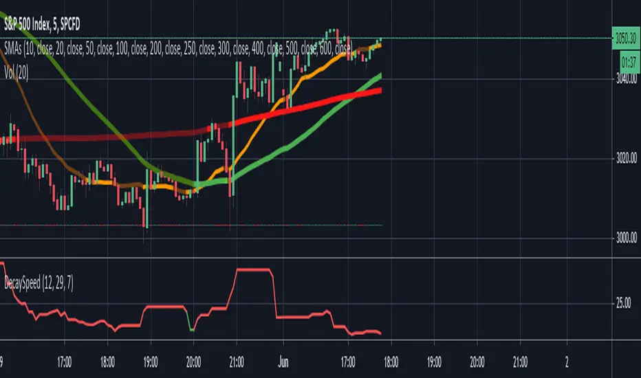
Options Decay Speed for 0DTEUse only for:
SPX, 5 minutes time frame
This indicator is complementing options 0DTE strategy - selling options for SPX index in the same day as they are expiring. Output of the indicator (red or green color of the curve) indicates whether is profitable to sell options at given moment at delta and VIX specified in the parameters. Changing parameter "Candles" is not recommended.
Main thought is that options expire with certain speed (theta decay) when stock doesnt move. When stock moves in unfavorable direction slowly enough, decay speed can compensate for disadvantage coming from option delta. Intuitively there must be certain speed of stock value change (expressed in stock value per 5 minutes) that is exactly compensating theta decay. This indicator calculates those two values (details below) and shows, where theta decay is faster than stock movement in the last hour and thus favorable to sell options.
Indicator gets its result from comparing two values:
1) volatility in the form of highest high and lowest low for past 12 candles (one hour in total) divided by 12 - meaning average movement of stock expressed in
2) speed of options value decay in form of combination of theta decay and option delta. Formulas are approximation of Black-Scholes model as Pine script doesnt allow for advanced functions. Approximations are accurate to 2 decimal points from market open to one hour before market close and will not indicate green when accuracy is not sufficient. Its value is also expressed in so its mutualy comparable.
My focus was not on code elegance but on practical usability.
Written by Ondřej Škop.
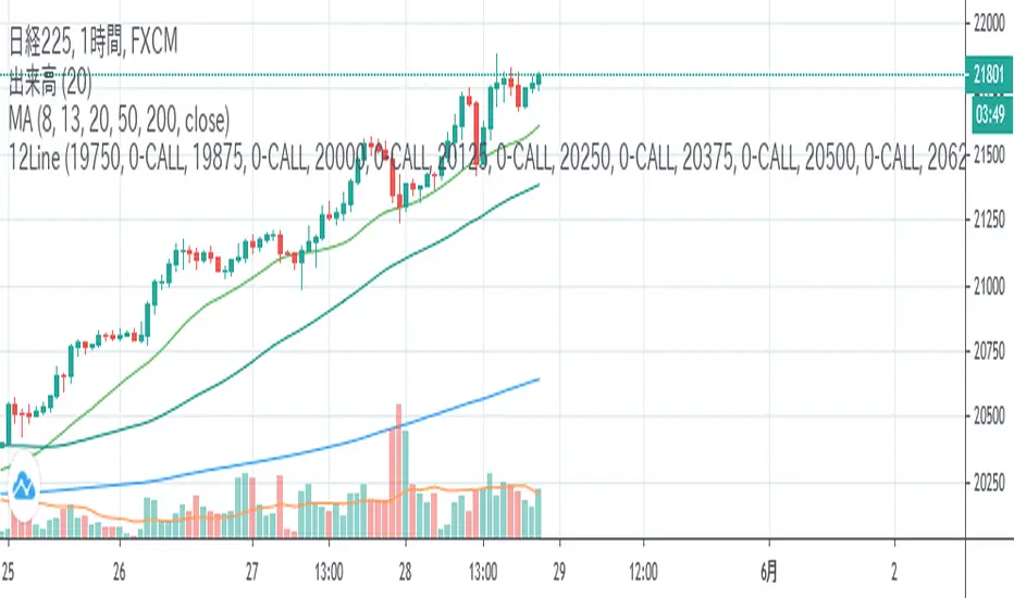
12LineA horizontal line is displayed during Nikkei 225 futures trading to help you draw a line quickly.
If you check the check box, you can display up to 12 lines of 6 types at the entered price.
日経平均先物取引時に水平ラインを表示し、素早いライン描画を助けます。
表示したい価格を入力し、チェックボックスをONにすると6種類の線を最大12本表示できます。
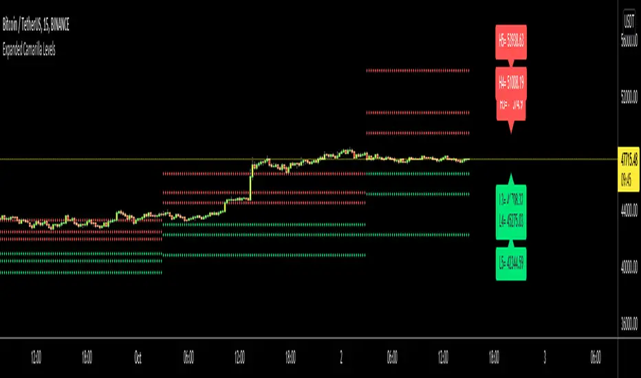
Expanded Camarilla LevelsHello Everyone,
The Expanded Camarilla Level s is introduced in the book " Secrets of a Pivot Boss: Revealing Proven Methods for Profiting in the Market " by Franklin Ocho a. I will not write a lot about the book, you should read it for yourself. There are many great ideas in the book, such using these levels, following trend, time price opportunity, Advanced Camarilla Concepts and much more.
The definition/formula of the levels defined in the book. ( actualy L1, L2, H1 and H2 levels are not used in the strategy, so not shown on the chart )
RANGE = highhtf - lowhtf
H5 = (HIGH/ LOW) * CLOSE
H4 = CLOSE + RANGE * 1.1/2
H3 = CLOSE+ RANGE * 1.1/4
H2 = CLOSE+ RANGE * 1.1/6
H1 = CLOSE+ RANGE * 1.1/12
L1 = CLOSE- RANGE * 1.1/12
L2 = CLOSE- RANGE * 1.1/6
L3 = CLOSE- RANGE * 1.1/4
L4 = CLOSE- RANGE * 1.1/2
L5 = CLOSE- (H5 - CLOSE)
Levels:
Strategy: you need to take care of the candles, as you can see there is bearish candle on first part, and Bullish Candle on second part!
Another Strategy:
An Example:
ENJOY!
.BXBT IndexThe current .BXBT index weighted as close as possible to BitMEX's with updates as BitMEX refreshes their index.
Difference between this and the script titled '2020 March 27 .BXBT Index': this one will receive updates because it doesn't have a date in its title.
Methodology
www.bitmex.com
"BitMEX Index Weights, assuming no constituent exchanges have been excluded due to Index Protection Rules, last updated 27 December 2019 at 12:00:05 UTC."
Binance: -
Bitstamp: 10.61%
Bittrex: 2.53%
Coinbase: 52.30%
Gemini: 6.89%
Huobi: -
Itbit: 4.21%
Kraken: 23.46%
Poloniex: -
ItBit's weight is combined with Gemini's due to ItBit not being on TradingView as of now. BITTREX:BTCUSD substituted with BITTREX:BTCUSDT*POLONIEX:USDTUSD to backfill because Bittrex only recently (late 2018) started to offer a fiat BTC/USD pair. Not that it matters since the index used in 2018 didn't include Bittrex if I remember correctly.
What is actually used for 27/12/2019 to 27/03/2020:
Binance: -
Bitstamp: 10.61%
Bittrex: 2.53%
Coinbase: 52.30%
Gemini: 11.10%
Huobi: -
Itbit: -
Kraken: 23.46%
Poloniex: -
Options:
Toggle candlesticks or close line
Change price source to be used for indicators
To be added: Change quarter to show indexes for different times, with labels that apply to the appropriate index used
Reasons to use this vs. the index itself: (not many)
It is helpful as a reference for other indicators or creation of an index.

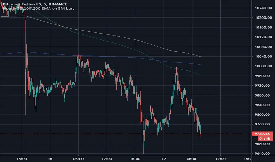
Hourly 50\100\200 EMA on 5M barsHello. This script was created for traders using a 5 minute timeframe. The script allows you to plot EMA from a higher level timeframe. Its formula includes the multiplication of the classical values of 50/100/200 EMA by 12, because in one hour it is 12 times for 5 minutes. You must use script only at 5M timeframe, because his interval is unique and not compare with other timeframes.
Often, an hourly EMA on a 5-minute timeframe becomes a strong level of support or price resistance. You can use this script on 5M timeframe with "daily 50/100/200 EMA" script on 1H timeframe for best scalping results.
Good luck in trading!
CCI strategy on OIL1HThis indicator is based on Commodity Channel Index.
It buys when CCI on period 200 is under -130 and it´s rising last 12 bars. It closes the position by hitting Take Profit, Stop Loss or opening short position.
It sells when CCI on period 200 is over 130 and it´s falling last 12 bars. It closes the position by hitting Take Profit, Stop Loss or opening short position.
This strategy seems to working just on USOIL on 1 hour chart. This can predict that it´s just luck and not proper strategy or indicator I would use for trading.
This script is just for educational purposes and that´s why the script is open. I will be happy if you will leave comment and try to come up with some ideas how to improve this strategy, so it can be used also on other commodities/forex pairs.
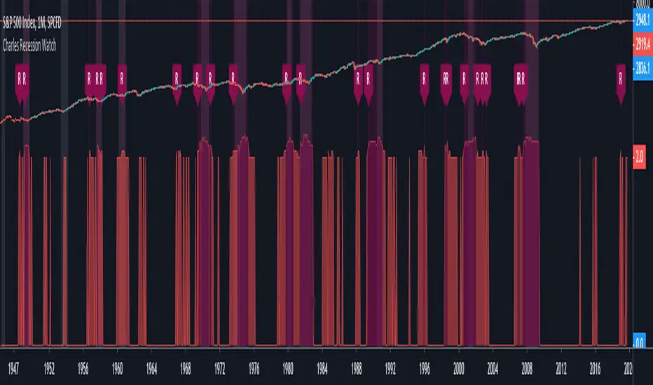
Charles Recession WatchThe “Recession Watch” indicator tracks 7 key economic metrics which have historically preceded US recessions. It provides a real-time indication of incoming recession risk.
This indicator gives a picture of when risk is increasing, and therefore when you might want to start taking some money out of risky assets.
All of the last seven recessions were preceded by a risk score of 3 or higher. Six of them were preceded by a risk score of 4 or higher. Unfortunately data prior to 1965 was inconsistent and prior recessions could not be considered.
Based on the indicator hit rate at successfully flagging recessions over the last 50 years, risk scores have the following approximate probabilities of recession:
- 0-1: Low
- 2: 25% within next 18 months
- 3: 30% within next 12 months
- 4-7: 50% within next 12 months
Note that a score of 3 is not necessarily a cause for panic. After all, there are substantial rewards to be had in the lead up to recessions (averaging 19% following yield curve inversion). For the brave, staying invested until the score jumps to 4+, or until the S&P500 drops below the 200day MA, will likely yield the best returns.
Notes on use:
- use MONTHLY time period only (the economic metrics are reported monthly)
- If you want to view the risk Score (1-7) you need to set your chart axis to "Logarithmic"
Enjoy and good luck!
ATR - Baby WhaleScript that shows you the ATR and 0.5 ATR.
You can use this to define your stop loss level when you see a SFP.
Standard setting is the 24 period ATR. You can use this for a 1h chart (24 hours in a day).
So when you play on a 5m chart, you can change the setting to 12 period (12 5m candles in 1 hour).

Saturn–Pluto Cycle
Indicator colors background of the chart in the following way:
Saturn - Pluto Cycle in conjunction: Blue
Saturn - Pluto Cycle in opposition: Yellow
While opposition periods are indicated according to the actual date ranges an opposition occurs, conjunctions last only for one day.
Conjunctions indicated with this indicator mark a period around the actual conjunction date.
The actual date a conjunction occurs is indicated in the script.
Following the dates which were considered for this indicator:
Dates of Saturn–Pluto Conjunctions
October 5, 1914 at 2° Cancer (recurrence on May 20, 1915)
August 11, 1947 at 13° Leo
November 8, 1982 at 27° Libra
January 12, 2020 at 22° Capricorn
Dates of Saturn–Pluto Oppositions
February 17, 1931 – December 13, 1931 at 19°–21° Capricorn–Cancer (conjunct their respective North and South Nodes)
April 23, 1965 – February 20, 1966 at 14°–17° Pisces–Virgo
August 5, 2001 – May 26, 2002 at 12°–16° Gemini–Sagittarius (conjunct the lunar nodes)

Consensio Vision MA - Tribute to Late Dean Tyler JenksA wonderful mentor, fearless leader and incredibly humble man, father alike and world renowned bitcoin influencer also known for the invention of robust money management system named consensio moving averages, Tribute to Late Dean Tyler Jenks who made this possible.
Explanation
this indicator make use of three simple moving averages, idea is to incrementally invest little by little in the bull market when all moving average is moving up
A more in-depth guide for consensio is available here
How to use this indicator?
This indicator plots weekly moving average on daily and/or hourly time frame, the basic idea is to see how smaller time frame like daily and hourly trend reacts to larger time frame like weekly moving averages and what are the possible support and resistance area on these smaller time frame and also to arrive at better entry points while doing that.
The name Consensio Vision is chosen cuz.. it's a free reminder to never loose long-term vision (in this case weekly trend) of where you're going
Consensio Vision MA - Tribute to Late Dean Tyler Jenks
Lucid's Principles Of Investing - These are principles foretold by Late dean tyler jenks.. he goes on to saying that those 12 principles will keep you out of trouble or will identify trouble or will identify your human behavioral problems
1. CASH IS KING - in terms of my investing principles is very simple cash is king, I would rather be in cash than any other asset class, unless an asset class is trending to the upside (or bull market) the cash is king
2. Market doesn't move in straight line - all asset classes trimmed up and down, as tyler goes on to say he dont believe in buy and hold strategy, i'm giving you the tools to get you out of market so you dont have drive down bear events like 2009 crash, he further suggests you sould react (or make decision) before a 10% drop in market.
3. Timeframe - trends are short days or weeks intermediate weeks or months and long months or years so principle number three is don't just talk about something is in a trend be precise are you talking about a short-term trend an intermediate term trend or a long-term trend...
just saying something is in a trend is irresponsible, you've got to identify your time frame
4. Wait! Bear market is different - cash is king and unless asset class is trending up there are times that you want to take advantage of a trend that is down but it is not the equivalent of investing in a trend that is up it is far more dangerous far more difficult it can be done but that's not one of the main principles, (also check rule number 7 as both are related)
5. Only long-term trends are investments - word trading is not really an investment term trading means buying or selling it has nothing to do with what you're attempting to achieve in terms of either speculation gambling investing ... those are not opportunities for investing because they're short or they're intermediate.. that doesn't mean that you can't speculate and have that turn into a position trade and have it turn into a possible swing trade and then have it turn in to an investment however be prepared once you've made an investment where that investment in a short or an intermediate term time frame to move against you
6. Never invest in a FOMO (fear of missing out)- loss of money loss of cash loss of wealth is not equivalent to a loss of opportunity
it is 100 times more important than a loss of opportunity
7. understand the importance of Percentage - a 50% gain is not an inverse equivalence of a 50% loss that is the single most important rule or principle that Lucid uses in determining when to get into or out of an investment and it goes back to number six that a loss of money is not equivalent to a loss of opportunity
8. all long-term trends are fundamentally based, repeat all long-term trends are fundamentally based
9. number nine is a corollary but it's separate all short and intermediate term trends are not fundamentally based, long term trends are not affected by news are not affected by headlines are not affected by company announcements or country announcements they are affected in the short in the intermediate term and therefore your probability of success goes way up as your timeframe frame goes longer
10. Fundamental vs technical - technical tools are invaluable in identifying trends fundamental tools are not invaluable in identifying trends - that's why technical analysis is so important it gives you something that fundamental analysis will never give you in time so technical a pro active mechanism or money management tool and fundamental is a lagging indicator hoever its what drives the market in log term
11. Profitability based on time aka VISION- I see even very sophisticated investors doing is they let the technical tools give them a signal on the short-termer intermediate-term and they believe because it's the tool that they're using that it's giving them an equivalent probability of success and it is not!
it's probability of success at the short-term is less than at the intermediate term and is less than at the long-term
12. the last one long-term trends are more important than intermediate which are more important than short term, tyler developed a scale where he ranks
long-term trend 5,
intermediate term trend 3,
short-term with a 1
(note: if you add both 3 & 1 its still smaller then 5)
if you add together my intermediate term weighting of 3 and the short term weighting of 1 that you do not equal the long term weighting of 5 that means that both the short and the intermediate term can be going in a direction but that does not negate the direction of the long term trend it's a simple way of looking at it and I use the word in number 12 important not simply to mean importance in terms of the weighting system but the probability of success of each of those 3
so if you're using a short term 15 minute 30 minute one hour signals or probability of success drops dramatically and therefore you've got to factor in where your stops are relative to that probability when you're in a long term trend a five waiting you don't need to use stops when you're in an intermediate term trend you've got to use stops and when you're in a short term trend you've got to use closed stops
official website- lucidinvestmentstrategies.com

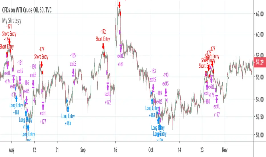
A.I.Driven TradersAI Model Trades for 20190612The entry and exit levels here are NOT derived from any specific indicator but are coming from our A.I. driven proprietary models.
This is an attempt at exploring the trading community here at TradingView and sharing our daily trading plans published at our site with the community here in the form a Pine Script - just starting and learning this platform. Please help point out any obvious errors or gotchas committed in the scripts. Thanks and have a great trading day!
**** The Trading Plan Published for today ****
>>>> Medium-Frequency Models: <<<<< For today, Wednesday 06/12, our medium-frequency models indicate using the 2895 as a pivot point - opening a long on a break above 2895, and opening a short on a break below 2895 (wait for a close on at least a five minute chart to determine the break), both sides with a 9-point trailing stop.
Note: For the trades to trigger, the breaks should occur during the regular session hours starting at 9:30am ET. By design, these models do NOT open any new positions after 3:45pm. Only one open position at any given time.
>>>>> Aggressive Intraday Models: <<<<< For today, Wednesday 06/12, our aggressive intraday models indicate going long on a break above 2892 or 2875 with an 6-point trailing stop, and going short on a break below 2887 or 2878 with an 8-point trailing stop.
Note: For the trades to trigger, the breaks should occur during regular session hours starting at 9:30am ET. Due to the intraday nature of these aggressive models, they indicate closing any open trades at 3:55pm and remaining flat into the session close. No opening of new positions after 3:45pm. Only one open position at any given time.

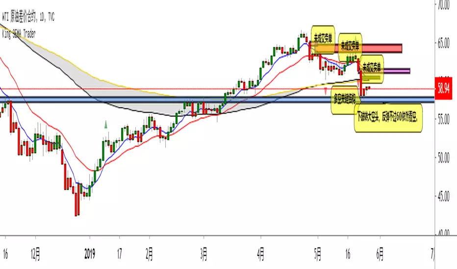
Edward EMA 8-21-89-144Explain the application of moving averages through the disk surface:
When the price runs above 89, it only looks for the buy signal.
When the price runs below 89, it only looks for sell signals.
The first step up through the 89 moving average after the first confirmation can buy homeoply,
The first pull down after crossing the 89 moving average for the first time confirms that it can be sold in line with the trend.
Price horizontal finishing, moving average frequently across the field observation.
The yellow area in the interval from 8 to 21 is the homeopathic warehouse addition signal.
When the price is above the 89 moving average, the k-line closes below the 21-day moving average as a callback signal
Prices below the 89 ema close above the 21 - day ema as a rebound signal
After the correction and rebound signals come out, we should make half of the profit and the other half of the stop loss in the break-even place.
Moving average is very suitable for the trend of strong varieties, is not suitable for volatile market.
Only at the end of the shock market moving average upward or downward divergent when it is possible to be used.
1. Repeatedly entangle the mean line of horizontal disk stage and observe it from the field
2. Sell the three EMA moving averages when they can't exceed 89EMA with downward crossing
3, many times can not break the new low when prices go sideways profit
4. Buy when the price reaches 89EMA after the convergence of triangle 3 is broken
5, the Angle of price rise slowed and closed below the 21 moving average when profit
6. Left field observation during transverse oscillation.
Sit tight while news or data cause prices to fall quickly
8. Buy when the price triangle breaks through the 89 moving average upward
9, the price does not rise to slow down when the horizontal closed below the 21 moving average when profit
10, price horizontal shock finishing at the same time the average line also transverse finishing field observation
11, the price of the triangle after finishing through the 89 moving average to buy.At this point all the averages have turned up
12, the second time can not break through the new high when the negative line can profit
13, the price of the first time in the same period of time through 89 after the first step back can be re-bought.
通过盘面讲解均线运用:
价格在89上面运行时时只找买入信号、
价格在89下面运行时只寻找卖出信号、
第一次向上穿过89均线后的第一次回踩确认可以顺势买入、
第一次向下穿过89均线后的第一次回抽确认可以顺势卖出、
价格横盘整理,均线频繁穿越时离场观察。
8-21区间里面黄色区域为顺势加仓信号,
价格在89均线上面时K线收盘在21天均线下面时为回调信号
价格在89均线下面时K线收盘在21天均线上面时为反弹信号
在回调和反弹信号出来之后我们应该获利一半的头寸,另外一半止损放到盈亏平衡的地方。
均线非常适合趋势性很强的品种,并不适合震荡行情。
只有在震荡行情结束时均线向上或向下发散时才有被运用的可能。
1、横盘阶段均线反复纠缠,离场观察
2、三条EMA均线向下交叉回抽无法超越89EMA时卖出
3、多次不能破新低时价格走横时获利
4、价格在3处三角形收敛被突破后站上了89EMA时买入
5、价格上涨角度变缓并收盘在21均线下面时获利
6、横盘震荡时离场观察。
7、见死不救新闻或数据导致价格快速下跌时观望
8、价格三角形向上突破时穿过89均线时买入
9、价格不升减速走横时收盘于21均线下面时获利
10、价格横盘震荡整理同时均线也横向整理时离场观察
11、价格突破三角形整理后重新穿过89均线时买入。此时所有均线已经向上翘头
12、第二次不能突破新高时收阴线可以获利
13、价格在同一个时间周期内第一次穿过89以后的第一次回踩可以重新买入
14、89-144作为牛熊的分水岭。在89-144区域之下只考虑做空,89-144只考虑做多。如果89-144走横则以位置决定高位倾向空低位倾向多。
15、K线会因为指标的设置自动变成两个颜色块,绿色看涨,红色看跌。做趋势看K线颜色。牛市的红色可以当成入场K熊市绿色当成入场K
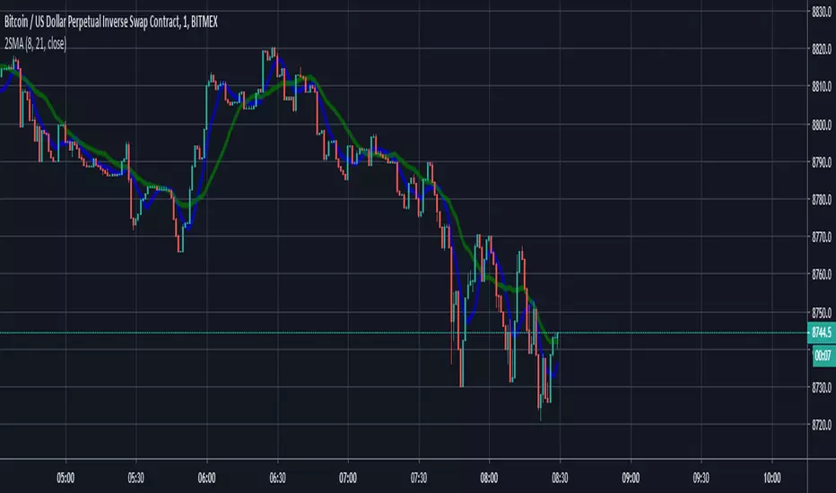
2 Exponential Moving AveragesThe Power of the 8 & 21 Day Moving Averages
Traders often ask me why I talk about the 8 & 21 day moving averages so much. Whether you see me on CNBC, Twitter, or the Virtual Trading Floor®, odds are you'll see me talking about them.
It's because these moving averages are the most accurate short-term road map I've found.
www.t3live.com
Complete EMA/SMA/BOLL setWhen you are on a simple plan and can't afford all the indicators... why not get them all in one!
Here are the main EMA's that I use on a day trading basis.. and no I don't have them all on at once!
I'm a big fan of the 12/26 EMA's on ALL time frames, however I sometimes just like to look at the 4 hourly chart. Problem is that I can't see the 12/26 Daily EMA's ?????
Well, with this tool you can.. just overlay the 'Dto4-ema12' etc
Also overlay weekly too if you feel the need!
PS: Threw the Bollinger Bands in there too, just for shits and giggles.
Enjoy!

Investing - Weekly EMA's mapped to Daily ChartWhen there isn't enough time in your day to day-trade, yet you want to utilise all the technical analysis skills you have... why not make a long term investing or swing trading indicator set to help you along the way!
So I did....
When it comes to long term investing and swing trading, I often find the weekly 12/26/52 EMA's do a great job in capturing the main market swings from bull to bear.
However, I like to use the Daily chart to see the candle patterns and shapes with more detail and divergences often show up better on the daily chart.
So I have decided to combine the two!
I have basically taken the EMA 12/26/52 from the weekly and transferred them over to the daily (mathematically they are not exact, but for me they are close enough).
I have also developed a simple scale in / scale out strategy for using these exponential moving averages. It isn't as simple as buying in on each signal, however I use my own special strategy to take advantage of the alerts.
Enjoy!

Simple Alt Coin Strategy - EMA and MACD w/Profit and StopThis script prints BUY and SELL signals based on settings you input. I use it to save time while scrolling through charts deciding what alts I want to look at.
BUY SIGNALS
Positive EMA Crossover
Positive MACD Crossover
Single Candle Gains
SELL SIGNALS
Profit Capture
Stop Loss
I don't trade based just on the BUY or SELL from this strategy, but I have found that these indicators do very well well looking at the large cap alt coins. It backtests well.
Default Settings EMA 5/12/50, MACD 9/12/26, Single Candle Gain 10%, Stop 10%, Profit Capture 45%

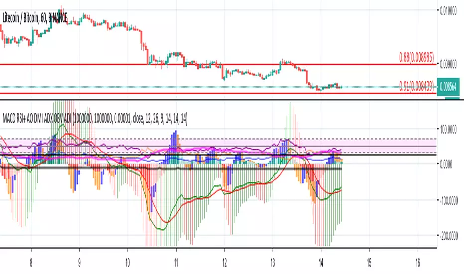
[astropark] MACD, RSI+, AO, DMI, ADX, OBV, ADI//******************************************************************************
// Copyright by astropark v4.1.0
// MACD, RSI+, Awesome Oscillator, DMI, ADX, OBV, ADI
// 24/10/2018 Added RSI with Center line to have clear glue of current trend
// 10/12/2018 Added MACD
// 13/12/2018 Added multiplier for MACD in order to make it clearly visible over RSI graph
// 11/01/2019 Added Awesome Ascillator (AO)
// 11/01/2019 Added Directional Movement Index (DMI) with ADX
// 14/01/2019 Added On Balance Volume (OBV)
// 14/01/2019 Added Accelerator Decelerator Indicator (ADI)
//******************************************************************************
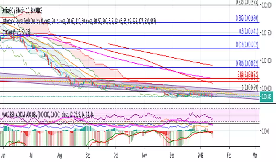
[astropark] MACD, RSI+, Awesome Oscillator, DMI, ADX, OBV//******************************************************************************
// Copyright by astropark v4.0.0
// MACD, RSI+, Awesome Oscillator, DMI, ADX, OBV
// 24/10/2018 Added RSI with Center line to have clear glue of current trend
// 10/12/2018 Added MACD
// 13/12/2018 Added multiplier for MACD in order to make it clearly visible over RSI graph
// 11/01/2019 Added Awesome Oscillator (AO)
// 11/01/2019 Added Directional Movement Index (DMI) with ADX
// 14/01/2019 Added On Balance Volume (OBV)
//******************************************************************************
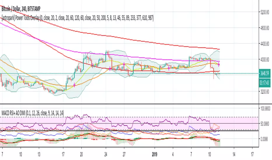
[astropark] MACD, RSI+, Awesome Oscillator, DMI with ADX//******************************************************************************
// Copyright by astropark v3.1.0
// MACD, RSI+, Awesome Oscillator, DMI, ADX
// 24/10/2018 Added RSI with Center line to have clear glue of current trend
// 10/12/2018 Added MACD
// 13/12/2018 Added multiplier for MACD in order to make it clearly visible over RSI graph
// 11/01/2019 Added Awesome Ascillator (AO)
// 11/01/2019 Added Directional Movement Index (DMI) with ADX
//******************************************************************************
[astropark] MACD, RSI+, Awesome Oscillator//******************************************************************************
// Copyright by astropark v3.0.0
// MACD, RSI+, Awesome Oscillator
// 24/10/2018 Added RSI with Center line to have clear glue of current trend
// 10/12/2018 Added MACD
// 13/12/2018 Added multiplier for MACD in order to make it clearly visible over RSI graph
// 11/01/2019 Added Awesome Ascillator (AO)
//******************************************************************************
