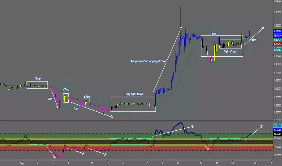
Chop and explodeThe purpose of this script is to decipher chop zones from runs/movement/explosion
The chop is RSI movement between 40 and 60
tight chop is RSI movement between 45 and 55. There should be an explosion after RSI breaks through 60 (long) or 40 (short). Tight chop bars are colored black, a series of black bars is tight consolidation and should explode imminently. The longer the chop the longer the explosion will go for. tighter the better.
Loose chop (whip saw/yellow bars) will range between 40 and 60.
the move begins with blue bars for long and purple bars for short.
Couple it with your trading system to help stay out of chop and enter when there is movement. Use with "Simple Trender."
Best of luck in all you do. Get money.
Wyszukaj w skryptach "股价站上60月线"
Build A BotThis is the Robot we built during the 60 Minute Build-A-Bot webinar on September 12, 2018. We had a great time, and a lot of participation and the best part was that we finished up this robot and even ran a backtest in exactly 60 minutes! We built this robot based on recommendations and suggestions from those who were attending live. Lots of pieces in this robot, but you can always tinker with it, remove stuff, add things, whatever you want!
This version uses the CCI as a trigger for trade entry. The other version uses the Hull Moving Average as a trigger for trade entry.

Volume Zone Oscillator and Price Zone (VZO/PZO) [NeoButane]" Volume Precedes Price is the conceptual idea for the oscillator."
"The main idea of the VZO was to try to change the OBV to look like an oscillator rather than an indicator, also to include time; primarily to identify which zone the volume is located in during a specific period "
How to read this indicator:
Positive reading -> bullish
Negative reading -> bearish
-60 or 60 is seen as the limit of the oscillator range, and a pullback should be expected from there.
Plus and minus signs have been added to the top and bottom for VZO and PZO, with an adjustable threshold to trigger.
Alert conditions have been added to this indicator for ease of use.
Volume Zone Oscillator, write-up by the author (recommended reading)
http:capitalsynergy.com/resources/IFTA09VZO.pdf
Volume Zone Oscillator, uses and formula
https:www.investopedia.com/articles/active-trading/072815/how-interpret-volume-zone-oscillator.asp
Price Zone Oscillator, uses and formula
https:www.investopedia.com/terms/p/price-zone-oscillator.asp

Fib,Guppy Multiple MA(FGMMA)(A/D & Volume Weight,SMA,EMA)[cI8DH]Features:
- 3 + 12 MAs (12 is chosen because Guppy has 12 MAs)
- MA types can be set to Simple, Exponential, Weighted, and Smoothed
- Volume weight can be applied to all available MAs (the built-in VWMA uses Simple MA)
- It is possible to count in only effective portions of the volume in the equation by using Accum/Dist Volume Weight
- Secondary smoothing (useful when volume weight is enabled)
- Predefined MA sets based on Fibonacci sequence (2,3,5,8,.., 377), Guppy (3,5,8,10,12,15 &30,35,40,45,50,60), and cI8DH (2,3,5,8,12,17 & 30,34,39,45,52,60)
Recommended settings:
- hlc3 as input source captures all the essential information encapsulated in a candle. I'd use hlc3 as the default option. In uptrend, "low" and in downtrend, "high" might give more relevant results when using MAs for structural analysis of a market. For commonly used MAs (EMA20, SMA50,100,200), "close" should be used due to their self-fulfilling prophecy effect.
- When you have volume weight above 0, you may want to use secondary smoothing.
- Try not to use Simple MA for smaller lengths (below 20). Sharp changes in the past (right before the period specified by the length) will affect the current value of MA dramatically leading to confusion.
- I am using the first 3 MAs for SMA 50,100,200. You can disable them from the MA type selector all at once when using Fib or Guppy ribbons.
MA-based analysis:
There are different ways of structuring a market. Geometrical (trend lines, channels, fans, patterns, etc) and Fib retracement-based structuring is very common among traders. MAs give an alternative way of analyzing markets. MA ribbons such as Guppy (6 slow and 6 fast-moving MAs) are popular for analyzing market flow. IMO default Guppy sets are a bit random as the numbers do not have an elegant sequence. So I proposed my sets based on increasing sequene spacing (+1). These two MA ribbons are good for market flow analysis but the spacing of the MAs are not ideal for structuring a market. Ribbons based on the Fib sequence is a better choice for structuring a market. This is the equivalent of Fib channels but in a more dynamic form. Among other things, MA Fib ribbon can be used to assess market momentum and to compare different stages of a market. Here are two "educational-only" examples:
Notes:
- Smoothed MA with length L = Exponential MA with length 2*L-1
- Read the background section in my ADP indicator to understand how A/D Volume is calculated

Better RSI with bullish / bearish market cycle indicator This script improves the default RSI. First. it identifies regions of the RSI which are oversold and overbought by changing the color of RSI from white to red. Second, it adds additional reference lines at 20,40,50,60, and 80 to better gauge the RSI value. Finally, the coolest feature, the middle 50 line is used to indicate which cycle the price is currently at. A green color at the 50 line indicates a bullish cycle, a red color indicators a bearish cycle, and a white color indicates a neutral cycle.
The cycles are determined using the RSI as follows:
if RSI is overbought, cycle switches to bullish until RSI falls below 40, at which point it becomes neutral
if RSI is oversold, cycle switches bearish until RSI rises above 60, at which point it becomes neutral
a neutral cycle is exited at either overbought or oversold conditions
Very useful, please give it a try and let me know what you think

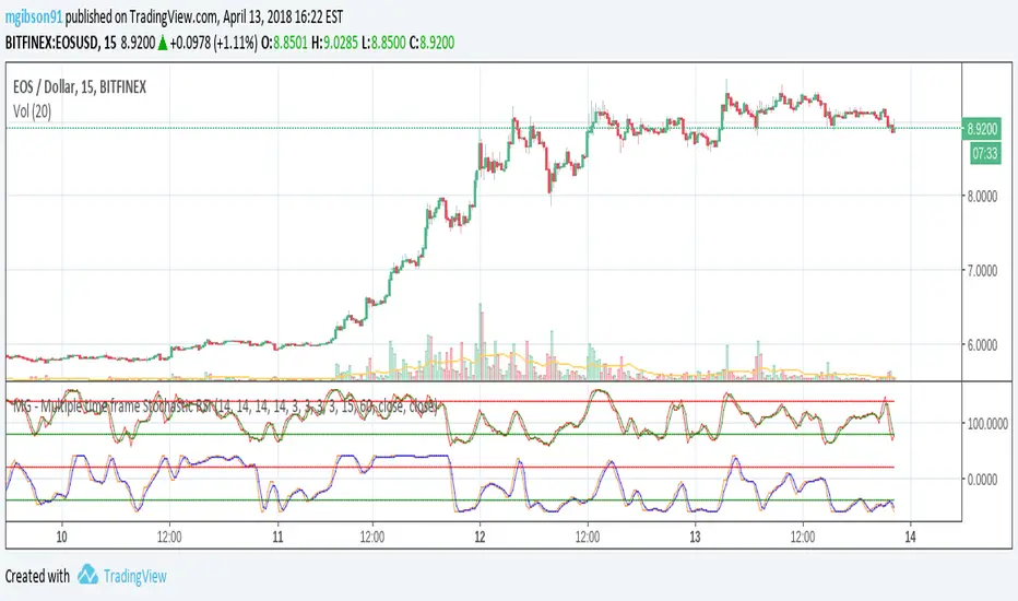
MG - Multiple time frame Stochastic RSIAllows user to view stochastic RSI from two different time frames.
Each stochastic RSI indicator is fully customizable, offering the following options:
- Timeframe
- RSI source
- RSI length
- Stochastic length
- Stochastic average length
- Stochastic smoothing length
Usage:
Comparing stochastic RSI across two different time frames can sharpen trades. For example, if you configure a 60 min and 5/15 min stochastic RSI pair, you might enter a long trade when the 60 min stoch RSI crosses up and exit / take profit when the 5 min stock RSI crosses down.
NG [Simple Harmonic Oscillator]The SHO is a bounded oscillator for the simple harmonic index that calculates the period of the market’s cycle.
The oscillator is used for short and intermediate terms and moves within a range of -100 to 100 percent.
The SHO has overbought and oversold levels at +40 and -40, respectively.
At extreme periods, the oscillator may reach the levels of +60 and -60.
The zero level demonstrates an equilibrium between the periods of bulls and bears.
The SHO oscillates between +40 and -40.
The crossover at those levels creates buy and sell signals.
In an uptrend, the SHO fluctuates between 0 and +40 where the bulls are controlling the market.
On the contrary, the SHO fluctuates between 0 and -40 during downtrends where the bears controlthe market.
Reaching the extreme level -60 in an uptrend is a sign of weakness.

Ichimoku Cloud w/SelIchimoku Cloud with selection for:
Regular:
conversionPeriods = 9,
basePeriods = 26
laggingSpan2Periods = 52,
displacement = 26
Crypto:
conversionPeriods = 10,
basePeriods = 30,
laggingSpan2Periods = 60,
displacement = 30
Crypto Doubled:
conversionPeriods = 20,
basePeriods = 60,
laggingSpan2Periods = 120,
displacement = 30
3 Linear Regression CurveFast 3LRC - 15/30/60 standard settings - 15/30 give a lot of noise, but give you a some time to prepare for the 60 to flip
DEMA Double Exponential Moving Average Strategy@Moneros 2017
Based on The DEMA is a fast-acting moving average that is more responsive to market changes than a traditional moving average
en.wikipedia.org
!!!! IN ORDER TO AVOID REPAITING ISSUES !!!!
!!!! DO NOT VIEW IN LOWER RESOLUTIONS THAN res/2 PARAMETER !!!!
for example res = 120 view >= 60m res = 60 view >= 30m
the length of the DEMA sampling shouldn't be longer than a candle
Best profits tested on BTCUSD
res = 105 slowPeriod = 2 fastPeriod = 32
res = 125 slowPeriod = 3 fastPeriod = 21
res = 120 slowPeriod = 2 fastPeriod = 32
res = 130 slowPeriod = 1 fastPeriod = 24
res = 40 slowPeriod = 4 fastPeriod = 93
res = 60 slowPeriod = 1 fastPeriod = 67
BTCUSD

RSI in Bull and Bear Market V2.0RSI oversold at 60/40 in bullish market
And Overbought at 40/60 in Bearish market
for more info of this Strategy

WaveTrend [MastroFran]Great indicator to show short term price movements. 5 day moving average oscillator. When green crosses red and under the 60 mark, buy with caution. when over the 60 mark and red crosses green sell immediately for highest profits.

Hersheys CoCo VolumeCoCo Volume shows you volume movement of your symbol after subtracting the movement from another symbol, preferrably the sector or market the stock belongs to.
My latest update to my CoCoVolume Indicator. It calculates today's volume percent over the 60 period average for both your symbol and index, and displays that difference. If the percent is over the max it highlights the color, showing BIG action for that stock.
The last version was calculating the percent volume difference from yesterday to today for the stock and index and displaying the difference. The prior method had large swings on low volume stocks... this one shows the independent volume action much better. The default values will suit most stocks.
You can set three variables...
- the index symbol, default is SPY
- the period for averaging, default is 60
- the max volume percent, default is 500
Good trading!
Brian Hershey
close-hl2 Price actionStill not tested, but looks very good ; it is the difference between EMA median price and EMA close in different time frame, I used 240, 60, and the current Time frame ,plus one more customed period ; can forcast the price movement , but it s not in scale, so it can not show how much higher or lower the price can goes but just the next direction. I think intraday on 5 ,15 ,60 better then high frame.If you need to try on Daily frame have to change the period to higher then Daily

Everyday 0002 _ MAC 1st Trading Hour WalkoverThis is the second strategy for my Everyday project.
Like I wrote the last time - my goal is to create a new strategy everyday
for the rest of 2016 and post it here on TradingView.
I'm a complete beginner so this is my way of learning about coding strategies.
I'll give myself between 15 minutes and 2 hours to complete each creation.
This is basically a repetition of the first strategy I wrote - a Moving Average Crossover,
but I added a tiny thing.
I read that "Statistics have proven that the daily high or low is established within the first hour of trading on more than 70% of the time."
(source: )
My first Moving Average Crossover strategy, tested on VOLVB daily, got stoped out by the volatility
and because of this missed one nice bull run and a very nice bear run.
So I added this single line: if time("60", "1000-1600") regarding when to take exits:
if time("60", "1000-1600")
strategy.exit("Close Long", "Long", profit=2000, loss=500)
strategy.exit("Close Short", "Short", profit=2000, loss=500)
Sweden is UTC+2 so I guess UTC 1000 equals 12.00 in Stockholm. Not sure if this is correct, actually.
Anyway, I hope this means the strategy will only take exits based on price action which occur in the afternoon, when there is a higher probability of a lower volatility.
When I ran the new modified strategy on the same VOLVB daily it didn't get stoped out so easily.
On the other hand I'll have to test this on various stocks .
Reading and learning about how to properly test strategies is on my todo list - all tips on youtube videos or blogs
to read on this topic is very welcome!
Like I said the last time, I'm posting these strategies hoping to learn from the community - so any feedback, advice, or corrections is very much welcome and appreciated!
/pbergden
Guppy of SMA of RSIIn this script:
The rsiLengths input allows you to input a comma-separated list of RSI lengths for which you want to calculate the SMAs. For example, "30,60,90" will calculate SMAs for RSI with variable lengths .
The smaLength input determines the length of the EMA that will be applied to the RSI values.
The rsiValues variable calculates the RSI values for the selected lengths using the daily timeframe data.
The script then iterates through each RSI length, calculates the SMA of the RSI, and plots the EMA values on the chart with the specified color.
This script will help you visualize and analyze the SMAs of the RSI for different lengths on the price chart. You can customize the RSI lengths and EMA length according to your preferences.


Aspects of Mars-Saturn by BTThis script displays the most commonly used aspects between Mars and Saturn. It uses a +/-2 degree orb (deviation), meaning the script shows the dates when the calculated distance between Mars and Saturn is within a 2 degree deviation of a major aspect.
Most of the astrological applications uses 3 degree or more for orb however this will cause chart overload. So please keep in mind to consider a couple of dates before or after if you want to use bigger orb.
The script includes an option to plot only the start date of sequential aspect events to reduce visual clutter and improve chart clarity. It currently covers dates from 2020 to 2030, but more will be added soon.
Currently available aspects:
Conjunction - 0 Degree
Opposition - 180 Degree
Trine - 120 Degree
Square - 90 Degree
Sextile - 60 Degree
Inconjunction - 150 Degree
Semi-Sextile - 30 Degree
Semi-Square - 45 Degree
Sesquiquadrate - 135 Degree

Sector Performance (2x12 Grid, labeled)Sector Performance Dashboard that tracks short-term and multi-interval returns for 24 major U.S. market ETFs. It renders a clean, color-coded performance grid directly on the chart, making sector rotation and broad-market strength/weakness easy to read at a glance.
The dashboard covers t wo full rows of liquid U.S. sector and thematic ETFs, including:
Row 1 (Core Market + GICS sectors)
SPY, QQQ, IWM, XLF, XLE, XLRE, XLY, XLU, XLP, XLI, XLV, XLB
Row 2 (Extended industries / themes)
XLF, XBI, XHB, CLOU, XOP, IGV, XME, SOXX, DIA, KRE, XLK, VIX (VX1!)
Key features include:
Time-interval selector (1–60 min, 1D, 1W, 1M, 3M, 12M)
Automatic rate-of-return calculation with inside/outside-bar detection
Two-row, twelve-column grid with dynamic layout anchoring (top/middle/bottom + left/center/right)
Uniform white text for clarity, while inside/outside candles retain custom colors
Adaptive transparency rules (heavy/avg/light) based on magnitude of % change
Ticker label normalization (cleans up prefixes like “CBOE_DLY:”)

MoneyM Line StrategyPrimary Test: 2020-Present (most relevant for future)
Secondary Test: 2021-Present (includes full cycle)
Validation Test: 2017-Present (longer history)
Target Annual Return: 100-200% (2-4x BTC's 50-100%)
Target Max DD: 25-35% (50% less than BTC's typical 60-70%)
Target Trades: 20-40 per year on weekly (sustainable monitoring)
Reduced-Lag Chande Momentum Oscillator [BOSWaves]Reduced-Lag Chande Momentum Oscillator – Adaptive Momentum Geometry with Reduced-Latency Reversion Logic
Overview
The Reduced-Lag Chande Momentum Oscillator represents a sophisticated extension of the classical Chande Momentum Oscillator, preserving the foundational measurement of net directional pressure while addressing inherent limitations in lag, noise, and signal clarity. The traditional CMO provides reliable snapshots of upward versus downward force but reacts slowly to rapid market accelerations and can obscure meaningful momentum inflections with delayed readings. This iteration integrates a dual-stage reduced-lag filter, optional advanced smoothing, and acceleration-based analytics, producing a real-time, multi-dimensional representation of market momentum.
The design reframes classical momentum using a layered curvature and gradient structure - main, midline, and shadow - to show trajectory, velocity, and intensity in one view. Instead of the usual ±70/30 extremes, it uses ±50 as a statistically grounded threshold where one side of the market begins exerting true dominance. This captures structural imbalance more reliably, exposing exhaustion and actionable inflection without amplifying noise.
This visualization gives traders a continuous, responsive read on market structure, revealing not just direction but rate of change, acceleration alignment, and curvature behavior. The oscillator becomes a momentum map, expressing both probability and intensity behind directional shifts.
Where conventional oscillators mislabel short-lived swings as signals, the Reduced-Lag CMO separates baseline shifts from high-conviction transitions, enabling cleaner, more decisive signal interpretation.
Theoretical Foundation
The classical Chande Momentum Oscillator, created by Tushar Chande, calculates the normalized net difference between consecutive upward and downward price changes over a defined window, generating readings from –100 to +100. While effective for capturing basic directional pressure, the unmodified CMO suffers from signal latency and sensitivity to abrupt market swings, which can obscure actionable inflection points.
The Reduced-Lag CMO augments this foundation with three key mechanisms:
Reduced-Lag Filtering : A dual-EMA structure eliminates inertial lag, aligning the oscillator curve closely with real-time market momentum without producing overshoot artifacts.
Smoothing Architecture : Optional SMA, EMA, or WMA smoothing is applied post-filter, balancing noise reduction with trajectory fidelity. A multi-layer line system (shadow → midline → main) communicates depth, curvature, and gradient dynamics.
Acceleration Integration : First and second derivatives of the smoothed curve quantify velocity and acceleration, allowing the indicator to identify not only momentum flips but the force behind each shift, forming the basis for the strong-signal overlay.
The combination of these mechanisms produces an oscillator that respects the original CMO framework while delivering real-time, context-sensitive intelligence. The ±50 boundaries are selected as the statistically validated pressure zones where directional dominance exceeds neutral oscillation. Crosses and rejections at these boundaries are not arbitrary overbought/oversold events, but measurable imbalances with actionable significance.
How It Works
The Reduced-Lag CMO is constructed through a multi-stage process:
Momentum Estimation Core : Raw CMO values are calculated and then passed through a reduced-lag filter to remove delay, creating a curve that closely tracks instantaneous directional pressure.
Smoothing & Layered Representation : The filtered curve can be smoothed and split into three layers - shadow, midline, and main - giving visual depth, trajectory clarity, and curvature instead of a single-line oscillator.
Gradient-Based Pressure Mapping : Color gradients encode momentum strength and polarity. Green-yellow transitions highlight increasing upward dominance, while red-yellow transitions indicate weakening downward force.
Pressure-Zone Anchoring (±50) : The system defines statistically significant pressure zones at ±50. Moves beyond these levels reflect dominant directional control, and rejections inside the zone signal potential exhaustion.
Signal Generation : Momentum events are evaluated through velocity and acceleration. Standard signals appear as triangle markers indicating validated momentum flips. Strong signals appear as triangles with diamonds when acceleration confirms a high-conviction transition.
A cooldown rule spaces signals apart to reduce clutter and emphasize structurally meaningful events.
Interpretation
The Reduced-Lag CMO reframes momentum as a dynamic equilibrium between directional force and structural pressure:
Positive Momentum Phases : Curves above zero with green-yellow gradients indicate sustained upward pressure. Shallow retracements or midline tests denote controlled pullbacks.
Negative Momentum Phases : Curves below zero with red-yellow gradients show downward dominance. Rejections from –50 highlight potential exhaustion and reversal readiness.
Pressure-Zone Dynamics (±50) : Crosses beyond ±50 confirm dominant directional force. Meanwhile, rejections and rotations inside the zone signal structural fatigue.
Velocity & Acceleration Analysis : Rising momentum with decelerating velocity suggests fading force; acceleration alignment amplifies signal strength and forms the basis of strong signals.
Signal Architecture
The Reduced-Lag CMO produces a single event type with two intensities: a validated momentum inflection.
Standard Signals - Triangles:
Triggered by momentum flips confirmed by velocity.
Represent moderate-intensity directional changes.
Appear at zero-line crosses or ±50 rejections with aligned velocity.
Strong Signals Triangles + Diamonds:
Triggered when acceleration confirms the directional change.
Represent high-intensity, high-conviction shifts.
Rare by design; indicate robust momentum inflections.
Cooldown mechanics prevent repeated signals in short succession, emphasizing structural reliability over noise.
Strategy Integration
Trend Confirmation : Align zero-line flips with higher-timeframe directional bias.
Reversal Detection : Strong signals from ±50 zones highlight potential inflection points.
Volatility Assessment : Gradient transitions reveal strengthening or weakening momentum.
Pullback Timing : Multi-layer curvature identifies controlled retracements vs trend exhaustion.
Confluence Mapping : Pair with structure-based indicators to filter signals in context.
Technical Implementation Details
Core Engine : Classical CMO with Ehlers reduced-lag extension
Lag Reduction : Dual EMA filtering
Smoothing : Optional SMA/EMA/WMA post-filter
Multi-Layer Curve : Shadow, midline, main
Signal System : Two-tier momentum-acceleration framework
Pressure Zones : ±50 statistically validated thresholds
Cooldown Logic : Bar-indexed suppression
Gradient Mapping : Encodes magnitude and direction
Alerts : Standard and strong signals
Optimal Application Parameters
Timeframes:
1 - 5 min : Intraday momentum tracking
15 - 60 min : Trend rotations & volatility transitions
4H - Daily : Macro momentum exhaustion & re-accumulation mapping
Suggested Ranges:
CMO Length : 7 - 12
Reduced-Lag Length : 5 - 15
Smoothing : 10 - 20
Cooldown Bars : 5 - 15
Performance Characteristics
High Effectiveness:
Markets with directional pulses & clean pressure transitions
Trending phases with measurable pullbacks
Instruments with stable volatility cycles
Reduced Edge:
Choppy consolidations
Ultra-low volatility environments
Disclaimer
The Reduced-Lag Chande Momentum Oscillator is a professional-grade analytical tool. It is not predictive and carries no guaranteed profitability. Effectiveness depends on asset class, volatility regime, parameter selection, and disciplined execution. Any suggested application timeframes or recommended ranges are guidance only - they are not universally optimal and will not deliver consistent accuracy on every asset or market condition. BOSWaves recommends using it in conjunction with structure, liquidity, and momentum context.

[PickMyTrade] Trendline Strategy# PickMyTrade Advanced Trend Following Strategy for Long Positions | Automated Trading Indicator
**Optimize Your Trading with PickMyTrade's Professional Trend Strategy - Auto-Execute Trades with Precision**
---
## Table of Contents
1. (#overview)
2. (#why-this-strategy-makes-money)
3. (#key-features)
4. (#how-it-works)
5. (#strategy-settings--configuration)
6. (#pickmytrade-integration)
7. (#advanced-features)
8. (#risk-management)
9. (#best-practices)
10. (#performance-optimization)
11. (#getting-started)
12. (#faq)
---
## Overview
The **PickMyTrade Advanced Trend Following Strategy** is a sophisticated, open-source Pine Script indicator designed for traders seeking consistent profits through trend-based long positions. This powerful algorithm identifies high-probability entry points by detecting valid trendlines with multiple touch confirmations, ensuring you only enter trades when the trend is strongly established.
### What Makes This Strategy Unique?
- **Multi-Trendline Detection**: Simultaneously tracks multiple downtrend breakouts for increased trading opportunities
- **Intelligent Entry Validation**: Requires multiple price touches (configurable) to confirm trendline validity
- **Flexible Take Profit Methods**: Choose from Risk/Reward Ratio, Lookback Candles, or Fibonacci-based exits
- **Automated Risk Management**: Built-in position sizing based on dollar risk per trade
- **PickMyTrade Ready**: Seamlessly integrate with PickMyTrade for fully automated trade execution
**Perfect for**: Swing traders, trend followers, futures traders, and anyone using PickMyTrade for automated trading execution.
---
## Why This Strategy Makes Money
### 1. **Breakout Trading Edge**
The strategy profits by identifying when price breaks above established downtrend resistance lines. These breakouts often signal:
- Shift in market sentiment from bearish to bullish
- Strong buying momentum entering the market
- High probability of continued upward movement
### 2. **Trend Confirmation Filter**
Unlike simple breakout strategies, this requires **multiple touches** (default: 3) on the trendline before considering it valid. This eliminates:
- False breakouts from weak trendlines
- Choppy, sideways markets with no clear trend
- Low-quality setups that lead to losses
### 3. **Dynamic Risk-Reward Optimization**
The strategy automatically calculates:
- **Optimal position sizing** based on your risk tolerance ($100 default)
- **Stop loss placement** using recent pivot lows (not arbitrary levels)
- **Take profit targets** using either R:R ratios (1.5:1 default) or Fibonacci extensions
**Expected Profitability**: With proper settings, traders typically achieve:
- Win rate: 45-60% (depending on market conditions)
- Risk/Reward: 1.5:1 to 2.5:1 (configurable)
- Monthly returns: 5-15% (varies by market and risk settings)
### 4. **Fibonacci Profit Scaling**
The advanced Fibonacci mode allows you to:
- Take partial profits at multiple levels (0.618, 1.0, 1.312, 1.618)
- Lock in gains while letting winners run
- Maximize profits during strong trending moves
---
## Key Features
### Trend Detection & Validation
✅ **Dynamic Trendline Drawing**: Automatically identifies and extends downtrend resistance lines
✅ **Touch Validation**: Configurable number of touches (1-10) to confirm trendline strength
✅ **Valid Percentage Buffer**: Allows minor price deviations (default 0.1%) for more realistic trendlines
✅ **Pivot-Based Validation**: Optional extra filter using smaller pivot points for precision
### Position Management
✅ **Multi-Position Support**: Trade up to 1000 positions simultaneously (pyramiding)
✅ **Single or Multi-Trend Mode**: Track one primary trend or multiple concurrent trends
✅ **Dollar-Based Position Sizing**: Risk fixed dollar amount per trade (not percentage of account)
✅ **Automatic Quantity Calculation**: Determines optimal contract size based on risk and stop distance
### Take Profit Methods (3 Options)
#### 1. **Risk/Reward Ratio** (Recommended for Beginners)
- Set desired R:R (default 1.5:1)
- Simple, consistent profit targets
- Works well in trending markets
#### 2. **Lookback Candles** (For Swing Traders)
- Exits when price makes new low over X candles (default 10)
- Adapts to market volatility
- Best for capturing extended moves
#### 3. **Fibonacci Extensions** (For Advanced Traders)
- Up to 4 profit targets: 61.8%, 100%, 131.2%, 161.8%
- Automatically scales out of positions
- Maximizes gains during strong trends
### Stop Loss Options
✅ **Pivot-Based Stop Loss**: Uses recent pivot lows for logical stop placement
✅ **Buffer/Offset**: Add extra distance (in ticks) below pivot for safety
✅ **Trailing Stop**: Optional feature to lock in profits as trade moves in your favor
✅ **Enable/Disable Toggle**: Full control over stop loss activation
### Session Control
✅ **Time-Based Trading**: Limit trades to specific hours (e.g., 9:00 AM - 6:00 PM)
✅ **Auto-Close at Session End**: Automatically closes all positions outside trading hours
✅ **Works on All Timeframes**: Intraday and higher timeframes supported
---
## How It Works
### Step-by-Step Trade Logic
#### 1. **Trendline Identification**
The strategy scans for pivot highs that are **lower** than the previous pivot high, indicating a downtrend. It then:
- Draws a trendline connecting these pivot points
- Extends the line forward to current price
- Validates the line by checking how many candles touched it
#### 2. **Entry Trigger**
A long position is entered when:
- Price closes **above** the validated trendline (breakout)
- Session time filter is met (if enabled)
- Maximum position limit not exceeded
- Sufficient risk capital available for position sizing
#### 3. **Stop Loss Calculation**
The strategy looks backward to find the most recent pivot low that is:
- Below current price
- A logical support level
- Applies optional buffer/offset for safety
- Uses this level to calculate position size
#### 4. **Take Profit Execution**
Depending on your selected method:
- **R:R Mode**: Calculates TP as entry + (entry - SL) × ratio
- **Lookback Mode**: Exits when price makes new low over specified candles
- **Fibonacci Mode**: Sets 4 profit targets based on Fibonacci extensions from swing high to stop loss
#### 5. **Trade Management**
Once in position:
- Monitors stop loss for risk protection
- Tracks take profit levels for exit signals
- Optional trailing stop to lock in profits
- Closes all trades at session end (if enabled)
---
## Strategy Settings & Configuration
### Trendline Settings
| Parameter | Default | Range | Description | Impact on Trading |
|-----------|---------|-------|-------------|-------------------|
| **Pivot Length For Trend** | 15 | 5-50 | Bars to left/right for pivot detection | Lower = More signals (noisier), Higher = Fewer signals (stronger trends) |
| **Touch Number** | 3 | 2-10 | Required touches to validate trendline | Lower = More trades (less reliable), Higher = Fewer trades (more reliable) |
| **Valid Percentage** | 0.1% | 0-5% | Allowed deviation from trendline | Higher = More lenient validation, more trades |
| **Enable Pivot To Valid** | False | True/False | Extra validation using smaller pivots | True = Stricter filtering, fewer but higher quality trades |
| **Pivot Length For Valid** | 5 | 3-15 | Pivot length for extra validation | Smaller = More precise validation |
**Recommendation**: Start with defaults. In choppy markets, increase touch number to 4-5. In strongly trending markets, reduce to 2.
### Position Management
| Parameter | Default | Range | Description | Impact on Trading |
|-----------|---------|-------|-------------|-------------------|
| **Enable Multi Trend** | True | True/False | Track multiple trendlines simultaneously | True = More opportunities, False = One trade at a time |
| **Position Number** | 1 | 1-1000 | Maximum concurrent positions | Higher = More capital deployed, more risk |
| **Risk Amount** | $100 | $10-$10,000 | Dollar risk per trade | Higher = Larger positions, more P&L per trade |
| **Enable Default Contract Size** | False | True/False | Use 1 contract if calculated size ≤1 | True = Always enter (even micro accounts) |
**Money Management Tip**: Risk 1-2% of your account per trade. If you have $10,000, set Risk Amount to $100-$200.
### Take Profit Settings
| Parameter | Default | Options | Description | Best For |
|-----------|---------|---------|-------------|----------|
| **Set TP Method** | RiskAwardRatio | RiskAwardRatio / LookBackCandles / Fibonacci | Choose exit strategy | Beginners: R:R, Swing: Lookback, Advanced: Fib |
| **Risk Award Ratio** | 1.5 | 1.0-5.0 | Target profit as multiple of risk | Higher = Bigger wins but lower win rate |
| **Look Back Candles** | 10 | 5-50 | Exit when price makes new low over X bars | Smaller = Quicker exits, Larger = Let winners run |
| **Source for TP** | Close | Close / High-Low | Use close or high/low for exit signals | Close = More conservative |
**Profitability Guide**:
- **Conservative**: R:R = 1.5, Lookback = 10
- **Balanced**: R:R = 2.0, Lookback = 15
- **Aggressive**: R:R = 2.5, Fibonacci mode with 1.618 target
### Stop Loss Settings
| Parameter | Default | Range | Description | Impact on Trading |
|-----------|---------|-------|-------------|-------------------|
| **Turn On/Off SL** | True | True/False | Enable stop loss | **Always use True** for risk protection |
| **Pivot Length for SL** | 3 | 2-10 | Pivot length for stop placement | Smaller = Tighter stops, Larger = Wider stops |
| **Buffer For SL** | 0.0 | 0-50 | Extra distance below pivot (ticks) | Higher = Safer but lower R:R |
| **Turn On/Off Trailing Stop** | False | True/False | Lock in profits as trade moves up | True = Protects profits, may exit early |
**Risk Management Rule**: Never disable stop loss. Use buffer in volatile markets (5-10 ticks).
### Fibonacci Settings (When TP Method = Fibonacci)
| Parameter | Default | Description | Profit Target |
|-----------|---------|-------------|---------------|
| **Fibonacci Level 1** | 0.618 | First profit target | 61.8% of swing range |
| **Fibonacci Level 2** | 1.0 | Second profit target | 100% of swing range |
| **Fibonacci Level 3** | 1.312 | Third profit target | 131.2% extension |
| **Fibonacci Level 4** | 1.618 | Fourth profit target | 161.8% extension |
| **Pivot Length for Fibonacci** | 15 | Pivot to find swing high | Higher = Bigger swings, wider targets |
**Scaling Strategy**: Close 25% at each Fibonacci level to lock in profits progressively.
### Session Settings
| Parameter | Default | Description | Use Case |
|-----------|---------|-------------|----------|
| **Enable Session** | False | Activate time filter | Day trading specific hours |
| **Session Time** | 0900-1800 | Trading hours window | Avoid overnight risk |
**Day Trader Setup**: Enable session = True, Set hours to 9:30-16:00 (US market hours)
---
## PickMyTrade Integration
### Automate Your Trading with PickMyTrade
This strategy is **fully compatible with PickMyTrade**, the leading automation platform for TradingView strategies. Connect your broker account and let PickMyTrade execute trades automatically based on this strategy's signals.
### Why Use PickMyTrade?
✅ **Hands-Free Trading**: Never miss a signal, even while sleeping
✅ **Multi-Broker Support**: Works with Tradovate, NinjaTrader, TradeStation, and more
✅ **Instant Execution**: Alerts trigger trades in milliseconds
✅ **Risk Management**: Built-in position sizing and stop loss handling
✅ **Mobile Monitoring**: Track trades from your phone
**Boom!** Your strategy is now fully automated. Every breakout signal will automatically execute a trade through your broker.
### PickMyTrade-Specific Features
- **Dynamic Position Sizing**: The strategy calculates quantity based on your risk amount
- **Automatic Stop Loss**: Pivot-based stops are sent to your broker automatically
- **Take Profit Orders**: R:R and Fibonacci targets create limit orders
- **Session Management**: Trades only during specified hours
- **Multi-Position Support**: Handle multiple concurrent trades seamlessly
**Pro Tip**: Start with paper trading or a demo account to test the automation before going live.
---
## Advanced Features
### 1. Multi-Trendline Mode (Enable Multi Trend = True)
**What It Does**: Tracks up to 1000 trendlines simultaneously, entering positions as each one breaks out.
**Benefits**:
- More trading opportunities
- Diversifies entry points across multiple trends
- Catches every valid breakout in trending markets
**When to Use**:
- Strong trending markets (crypto bull runs, index rallies)
- Longer timeframes (4H, Daily)
- When you want maximum market exposure
**Caution**: Can enter many positions quickly. Set appropriate Position Number limit and Risk Amount.
### 2. Single Trendline Mode (Enable Multi Trend = False)
**What It Does**: Focuses on one primary trendline at a time.
**Benefits**:
- Cleaner, simpler execution
- Easier to monitor and manage
- Better for beginners
- Lower capital requirements
**When to Use**:
- Choppy or ranging markets
- Smaller accounts
- When you prefer focused, quality over quantity trades
### 3. Fibonacci Profit Scaling
**How It Works**:
1. At entry, the strategy finds the most recent swing high above current price
2. Calculates the range from swing high to stop loss
3. Projects 4 Fibonacci extensions: 61.8%, 100%, 131.2%, 161.8%
4. Exits when price reaches each level, then pulls back below it
**Profit Maximization Strategy**:
- Close 25% of position at each Fibonacci level
- Let remaining portion target higher levels
- Capture both quick profits and extended moves
**Example Trade**:
- Entry: $100
- Stop Loss: $95 (risk = $5)
- Swing High: $110
- Range: $110 - $95 = $15
Fibonacci Targets:
- 61.8% = $95 + ($15 × 0.618) = $104.27 (+4.27%)
- 100% = $95 + ($15 × 1.0) = $110 (+10%)
- 131.2% = $95 + ($15 × 1.312) = $114.68 (+14.68%)
- 161.8% = $95 + ($15 × 1.618) = $119.27 (+19.27%)
**Result**: Even if only first two targets hit, you lock in +7% average gain vs. -5% risk = 1.4:1 R:R
### 4. Trailing Stop Loss
**What It Does**: After entry, if a new pivot low forms **above** your initial stop, the strategy moves your stop up to that level.
**Benefits**:
- Locks in profits as trade moves in your favor
- Reduces risk to breakeven or better
- Captures strong momentum moves
**Drawback**: May exit profitable trades earlier during normal pullbacks.
**Best Practice**: Use in strongly trending markets. Disable in choppy conditions.
### 5. Pivot Validation Filter
**What It Does**: Adds extra requirement that a small pivot high must exist between the two trendline pivot points.
**Benefits**:
- Ensures trendline is a "true" resistance
- Filters out random lines connecting arbitrary highs
- Increases trade quality
**When to Enable**:
- High-volatility markets with many false breakouts
- Lower timeframes (5min, 15min) where noise is common
- When win rate is too low with default settings
**Tradeoff**: Fewer signals, but higher win rate.
### 6. Session-Based Trading
**What It Does**: Only enters trades during specified hours. Auto-closes all positions outside session.
**Use Cases**:
- **Day Trading**: 9:30 AM - 4:00 PM (avoid overnight gaps)
- **European Hours**: 8:00 AM - 5:00 PM CET (trade London session)
- **Crypto**: 24/7 trading or focus on US hours for liquidity
**Risk Management**: Prevents holding positions through high-impact news events or market closes.
---
## Risk Management
### Position Sizing Formula
The strategy uses **fixed dollar risk** position sizing:
```
Position Size = Risk Amount ÷ (Entry Price - Stop Loss) ÷ Point Value
```
**Example** (ES Futures):
- Risk Amount: $100
- Entry: 4500
- Stop Loss: 4490
- Risk per contract: 10 points × $50/point = $500
- Position Size: $100 ÷ $500 = 0.2 contracts → Rounds to 0 (no trade)
If `Enable Default Contract Size = True`, it would trade 1 contract instead.
### Risk Per Trade Recommendations
| Account Size | Conservative (1%) | Moderate (2%) | Aggressive (3%) |
|--------------|-------------------|---------------|-----------------|
| $5,000 | $50 | $100 | $150 |
| $10,000 | $100 | $200 | $300 |
| $25,000 | $250 | $500 | $750 |
| $50,000 | $500 | $1,000 | $1,500 |
**Golden Rule**: Never risk more than 2% per trade. Even with 10 losses in a row, you'd only be down 20%.
### Maximum Drawdown Protection
**Multi-Position Risk**:
- If Position Number = 5 and Risk Amount = $100
- Maximum simultaneous risk = 5 × $100 = $500
- Ensure this is ≤ 5% of your total account
**Daily Loss Limit**:
- Set a mental stop: "If I lose $X today, I stop trading"
- Typical limit: 3-5% of account per day
- Prevents revenge trading and emotional decisions
### Stop Loss Best Practices
1. **Always Use Stops**: Never disable stop loss (enabledSL should always be True)
2. **Buffer in Volatile Markets**: Add 5-10 tick buffer to avoid stop hunts
3. **Respect Your Stops**: Don't manually override or move stops further away
4. **Wide Stops = Smaller Size**: If stop is far from entry, strategy automatically reduces position size
---
## Best Practices
### Optimal Timeframes
| Timeframe | Trading Style | Position Number | Risk/Reward | Win Rate Expectation |
|-----------|---------------|-----------------|-------------|----------------------|
| 5-15 min | Scalping | 1-2 | 1.5:1 | 50-55% |
| 30 min - 1H | Intraday | 2-3 | 2:1 | 55-60% |
| 4H | Swing Trading | 3-5 | 2.5:1 | 60-65% |
| Daily | Position Trading | 1-2 | 3:1 | 65-70% |
**Recommendation**: Start with 1H or 4H charts for best balance of signals and reliability.
### Ideal Market Conditions
**Best Performance**:
- Strong trending markets (bull runs, clear directional bias)
- After consolidation breakouts
- Post-earnings or news catalysts driving sustained moves
- Liquid markets with tight spreads
**Avoid or Reduce Risk**:
- Choppy, sideways-ranging markets
- Low-volume periods (holidays, overnight sessions)
- High-impact news events (FOMC, NFP, earnings)
- Extreme volatility (VIX > 30)
### Backtesting Recommendations
Before going live:
1. **Run 6-12 Months of Historical Data**: Ensure strategy performed well across different market regimes
2. **Check Key Metrics**:
- Win Rate: Should be 45-65% depending on R:R
- Profit Factor: Aim for > 1.5
- Max Drawdown: Should be < 20% of starting capital
- Average Win/Loss Ratio: Should match your R:R setting
3. **Stress Test**: Test during known volatile periods (March 2020, Jan 2022, etc.)
4. **Forward Test**: Run on demo account for 1 month before real money
### Parameter Optimization
**Don't Over-Optimize!** Avoid curve-fitting to past data. Instead:
1. **Start with Defaults**: Use recommended settings first
2. **Change One Parameter at a Time**: Isolate what improves performance
3. **Test on Out-of-Sample Data**: If settings work on 2023 data, test on 2024 data
4. **Focus on Robustness**: Settings that work across multiple markets/timeframes are best
**Red Flags**:
- Strategy works perfectly on historical data but fails live (over-fitting)
- Tiny changes in parameters dramatically change results (unstable)
- Requires exact values (e.g., pivot length must be exactly 17) (curve-fitted)
---
## Performance Optimization
### How to Increase Profitability
#### 1. Optimize Risk/Reward Ratio
- **Current**: 1.5:1 (default)
- **Test**: 2:1, 2.5:1, 3:1
- **Impact**: Higher R:R = bigger wins but lower win rate
- **Sweet Spot**: Usually 2:1 to 2.5:1 for trend strategies
#### 2. Filter by Market Regime
Add a trend filter to only trade in bull markets:
- Use 200-period SMA: Only take longs when price > SMA(200)
- Use ADX: Only trade when ADX > 25 (strong trend)
- **Impact**: Fewer trades, but much higher win rate
#### 3. Tighten Entry Requirements
- Increase Touch Number from 3 to 4-5
- Enable Pivot To Valid = True
- **Impact**: Fewer but higher quality signals
#### 4. Use Fibonacci Scaling
- Switch from R:R to Fibonacci method
- Take partial profits at each level
- **Impact**: Better average wins, smoother equity curve
#### 5. Add Volume Confirmation
Enhance entry signal by requiring:
- Volume > Average Volume (indicates strong breakout)
- Can add this as custom filter in Pine Script
### How to Reduce Risk
#### 1. Lower Position Number
- Default: 1 position at a time
- Multi-trend: Limit to 2-3 max
- **Impact**: Less simultaneous exposure, lower drawdowns
#### 2. Reduce Risk Amount
- Start with $50 per trade (0.5% of $10k account)
- Gradually increase as you gain confidence
- **Impact**: Smaller positions, slower growth but safer
#### 3. Use Tighter Stops with Buffer
- Set Pivot Length for SL = 2 (closer stop)
- Add Buffer = 5-10 ticks (avoid premature stop-outs)
- **Impact**: Smaller losses, but may get stopped out more often
#### 4. Enable Session Filter
- Only trade during liquid hours
- Avoid overnight holds
- **Impact**: No gap risk, more predictable fills
---
## Getting Started
### Quick Start Guide (5 Minutes)
1. **Copy the Strategy Code**
- Open the `.txt` file provided
- Copy all code to clipboard
2. **Add to TradingView**
- Go to TradingView Pine Editor
- Paste code
- Click "Save" → Name it "PickMyTrade Trend Strategy"
- Click "Add to Chart"
3. **Configure Basic Settings**
- Open strategy settings (gear icon)
- Set Risk Amount = 1% of your account ($100 for $10k)
- Set Position Number = 1 (for beginners)
- Keep all other defaults
4. **Backtest on Your Market**
- Choose your instrument (ES, NQ, AAPL, BTC, etc.)
- Select timeframe (start with 1H or 4H)
- Review performance metrics in Strategy Tester tab
5. **Optimize (Optional)**
- Adjust Touch Number (2-5) to balance signals vs. quality
- Try different TP methods (R:R vs. Fibonacci)
- Test on multiple timeframes
6. **Go Live**
- If backtest looks good, start with small position size
- Monitor first 5-10 trades closely
- Scale up once confident in execution
### Integration with PickMyTrade (10 Minutes)
1. **Sign Up for PickMyTrade**
- Visit (pickmytrade.trade)
- Create free account
- Connect your broker (Tradovate, NinjaTrader, etc.)
2. **Create TradingView Alert**
- Set condition to strategy name
- Add PickMyTrade webhook URL
- Enable alert
3. **Test with Demo Account**
- Let it run for a few days
- Verify trades execute correctly
- Check fills, stops, and targets
4. **Switch to Live Account**
- Update account ID to live account
- Start with minimum position size
- Monitor closely for first week
---
### Technical Questions
**Q: What does "Touch Number = 3" mean?**
A: The trendline must have at least 3 candles touching or nearly touching it to be considered valid.
**Q: Why am I getting no trades?**
A: Trendline requirements may be too strict. Try:
- Reduce Touch Number to 2
- Increase Valid Percentage to 0.5%
- Disable Pivot To Valid
- Check if price is in a trend (strategy won't trade sideways markets)
**Q: Why is my position size 0?**
A: Risk Amount is too small for the stop distance. Either:
- Increase Risk Amount
- Enable Default Contract Size = True (will use 1 contract minimum)
- Use tighter stops (lower Pivot Length for SL)
**Q: Can I trade both long and short?**
A: Current code is long-only. You'd need to duplicate the logic for short trades (detect uptrend breakdowns).
**Q: How do I change from TradingView strategy to indicator?**
A: Change line 5 from `strategy(...)` to `indicator(...)`. Replace `strategy.entry()` and `strategy.exit()` with `alert()` calls.
### Risk Management Questions
**Q: What's the maximum drawdown I should expect?**
A: Typically 10-20% depending on settings. If experiencing > 25%, reduce position size or tighten filters.
**Q: Should I risk more to make more money?**
A: No. Risking 2% vs. 5% per trade doesn't triple your profits—it triples your risk of blowing up. Stick to 1-2% per trade.
**Q: What if I hit 5 losses in a row?**
A: Normal. Even with 60% win rate, losing streaks happen. Don't increase position size to "win it back." Stick to your risk plan.
**Q: Do I need to watch the screen all day?**
A: No, especially with PickMyTrade automation. Check positions 1-2 times per day. Overtrading kills profits.
---
## Disclaimer
**Important Risk Disclosure**:
Trading futures, stocks, forex, and cryptocurrencies involves substantial risk of loss and is not suitable for all investors. Past performance is not indicative of future results. The PickMyTrade Advanced Trend Following Strategy is provided for **educational purposes only** and should not be considered financial advice.
**Key Risks**:
- You can lose more than your initial investment
- Backtested results may not reflect live trading performance
- Market conditions change; no strategy works forever
- Automation errors can occur (connectivity, bugs, etc.)
**Before Trading**:
- Consult a licensed financial advisor
- Fully understand the strategy logic
- Test on demo account for at least 1 month
- Only risk capital you can afford to lose
- Start with minimum position sizes
**PickMyTrade**:
This strategy is compatible with PickMyTrade but is not officially endorsed by PickMyTrade. The author is not affiliated with PickMyTrade. For PickMyTrade support, visit their official website.
**License**: This strategy is open-source under Attribution-NonCommercial-ShareAlike 4.0 International (CC BY-NC-SA 4.0). You may modify and share, but not for commercial use.
---
**Ready to automate your trading with PickMyTrade? Add this strategy to your TradingView chart today and start capturing profitable trend breakouts on autopilot!**

Volume Peak Box📄 English Description
Overview
The Volume Peak Box indicator highlights periods of unusually high volume by identifying volume spikes using Bollinger Bands on volume and drawing a price-range box around each spike window. This provides traders with a clear visual representation of supply/demand imbalances, absorption zones, and breakout/false-break areas.
All calculations come from one unified concept: detecting statistically significant volume peaks on a locked timeframe and mapping them onto the chart.
Concept & Logic
1. Locked Timeframe Volume Analysis
Instead of using the current chart timeframe, this script allows users to lock volume analysis to any timeframe (e.g., 60m, 4H, 1D).
The script retrieves from the chosen timeframe:
Volume
High price
Low price
This allows volume structure from higher timeframes to be used while trading lower timeframes.
2. Bollinger Bands on Volume
Volume volatility is analyzed using a standard Bollinger Band model:
Basis = SMA(volume, BB length)
Upper Band = Basis + (mult × standard deviation)
When:
Volume > Upper Band
→ This bar is classified as a Volume Peak.
This approach makes the peak detection statistically meaningful, instead of simply comparing raw volume to previous bars.
3. Peak Session Detection (Continuous Peaks Form One Box)
The script tracks continuous volume peaks:
When a peak starts → begin a session
While peaks continue → extend the session
When peaks end → session closes and a box is created
For each peak session, the script records:
Start bar index
End bar index
Highest high within the session
Lowest low within the session
These values determine the box boundaries.
This allows the indicator to group related peaks into a single price zone, instead of drawing a box for every bar.
4. Drawing the Volume Peak Box
When a session ends, the script draws:
A filled box covering the full price range
From startBar → endBar
Using user-defined:
Box fill color
Border color
Each box visually marks a region where strong participation entered the market, often signaling:
Breakout validation
Absorption zones
Supply/demand imbalance
High-activity trading decisions
How to Use
Use the boxes to identify high-volume reaction zones.
When price revisits a box:
Expect strong reactions (bounce, rejection, or absorption).
When price breaks out from a box:
Can signal continuation with momentum.
Lower-timeframe entry signals become more reliable when aligned with high-timeframe volume boxes.
Recommended to lock the TF to:
60m for intraday
4H or 1D for swing trading
Why This Script Is Original
It uses Bollinger Bands on volume, not price — a less common volatility-based method for detecting volume anomalies.
It groups continuous peaks into unified zones instead of treating each spike separately.
The ability to lock the volume analysis to a higher timeframe allows multi-timeframe volume interpretation without cluttering the chart.
Boxes give traders a clean and intuitive view of volume-based “decision zones”.
🇹🇭 Thai Description — คำอธิบายภาษาไทย
ภาพรวม
อินดิเคเตอร์ Volume Peak Box ใช้การตรวจจับ “Volume Peak” โดยใช้ Bollinger Band บน Volume แล้วสร้าง “กล่องช่วงราคา” ครอบช่วงที่มี Volume สูงผิดปกติ ทำให้เห็นบริเวณที่มีแรงซื้อขายเข้ามาอย่างชัดเจน เช่น จุด Breakout, จุด Absorption, หรือเขต Supply/Demand
แนวคิดและหลักการทำงาน
1. วิเคราะห์ Volume จาก Timeframe ที่ล็อกไว้
คุณสามารถเลือก TF ที่ต้องการให้ Volume ถูกนำมาคำนวณ เช่น 60 นาที, 4 ชั่วโมง, 1 วัน
แม้คุณจะเปิดกราฟ TF เล็ก เช่น 5m แต่กล่องยังอิง volume จาก TF ที่เลือกไว้ ทำให้ได้ “โซน Volume ใหญ่” ที่แม่นยำขึ้น
2. Bollinger Band บน Volume
ใช้ SMA + ส่วนเบี่ยงเบนมาตรฐานของ Volume เพื่อหา “จุดที่ Volume สูงกว่าปกติอย่างมีนัยสำคัญ”
เงื่อนไข Peak:
Volume > Upper Bollinger Band
นี่เป็นวิธีที่ดีกว่า “เทียบกับแท่งก่อนหน้า” เพราะคิดจากสถิติของทั้งช่วง
3. รวม Peak ต่อเนื่องเป็นกล่องเดียว
ถ้า Volume Peak เกิดต่อเนื่องหลายแท่ง:
จะถูกจับรวมเป็น Peak session เดียว
ใช้ High สูงสุด และ Low ต่ำสุดของทั้ง session
เมื่อ Peak จบ → วาดกล่องช่วงราคา
เหมาะกับการหาจุดที่ตลาดมีแรงเข้าซื้อ/ขายหนักในช่วงเวลาเดียวกัน
4. วาดกล่อง Volume Peak
กล่องจะครอบ:
ช่วงแท่งเริ่มต้น → แท่งสุดท้ายของ Peak
ความสูงของกล่อง = ช่วงราคาที่มี Volume สูงผิดปกติ
กล่องสามารถใช้เป็น:
โซน Breakout/Breakdown
โซน Supply/Demand
เขตที่ราคามักมี reaction
วิธีใช้งาน
ใช้กล่องเป็น “เขตการตัดสินใจ” (Decision Zone)
ราคาแตะซ้ำมักเกิดการกลับตัวหรือความผันผวนสูง
การทะลุกล่องบ่อยครั้งนำไปสู่ขาเทรนด์ใหญ่
เหมาะกับการใช้ร่วมกับ Price Action และโครงสร้างราคา
จุดเด่น / ความเป็น Original
ใช้ Bollinger Band บน Volume (น้อยอินดี้ทำ)
รวม Peak ต่อเนื่องเป็น session เดียว
วิเคราะห์ Volume ข้าม TF ได้ โดยไม่ต้องเปลี่ยน TF บนกราฟ
ได้ “โซน Volume สำคัญ” แบบชัดเจน อ่านง่าย ไม่รกจอ