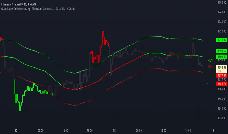
Quantitative Price Forecasting - The Quant ScienceThis script is a quantitative price forecasting indicator that forecasts price changes for a given asset.
The model aims to forecast future prices by analyzing past data within a selected time period. Mathematical probability is used to calculate whether starting from time X can lead to reaching prices Y1 and Y2. In this context, X represents the current selected time period, Y1 represents the selected percentage decrease, and Y2 represents the selected percentage increase. The probabilities are estimated using the simple average.
The simple average is displayed on the chart, showing in red the periods where the price is below the average and in green the periods where the price is above the average.
This powerful tool not only provides forecasts of future prices but also calculates the distribution of variations around the average. It then takes this information and creates an estimate of the average price variation around the simple average.
Using a mean-reverting logic, buying and selling opportunities are highlighted.
We recommend turning off the display of bars on your chart for a better experience when using this indicator.
Unlock the full potential of your trading strategy with our powerful indicator. By analyzing past price data, it provides accurate forecasts and calculates the probability of reaching specific price targets. Its mean-reverting logic highlights buying and selling opportunities, while the simple moving average displayed on the chart shows periods where the price is above or below the average. Additionally, it estimates the average variation of price around the simple average, giving you valuable insights into price movements. Don't miss out on this valuable tool that can take your trading to the next level
Probability
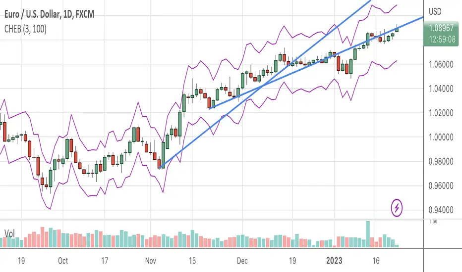
Chebyshevs BandsThis script calculates upper and lower bands using Chebyshev's inequality formula.
The main pros.: the band doesn't depend on particular distribution. It fits to any type of random variables. Also it allows to calculate bands for instruments with extremely high volatility.
Cons.: formula provides a rough estimation in some special cases like lognormal distribution.
Bayesian BBSMA + nQQE Oscillator + Bank funds (whales detector)Three trend indicators in one. Fork of Gunslinger2005 indicator, with a fix to display the nQQE oscillator correctly and clearly, and converted to pinescript v5 (allowing to set a different timeframe and gaps).
How to use: Essentially, nQQE is a long term trend indicator which is more adequate in daily or weekly timeframe to indicate the current market cycle. Banker Fund seems better suited to indicate current local trend, although it is sensitive to relief rallies. Bayesian BBSMA is an awesome tool to visualize the buildup in bullish/bearish sentiment, and when it is more likely to get released, however it is unreliable, so it needs to be combined with other indicators.
Please show the original indicators some love:
Bayesian BBSMA:
nQQE:
L3 Banker Fund Flow Trend:
Originally mixed together by Gunslinger2005:

Probability Cloud BASIC [@AndorraInvestor]🔮☁️
This is the BASIC version of the PROBABILITY CLOUD indicator.
It is an evolution beyond traditional standard deviation probabilistic indicators only using bands or channels.
The new PROBABILITY CLOUD graphic representation with customizable transparent layers is based on -2 / +2 standard deviation calculated using 20 fixed predetermined time periods, and is available in several calculation MODES:
SMA , EMA , WMA , VWMA , VWMA & VAWMA
The indicator is designed to let the trader visually understand the probabilistic depth of past, present and future price action, and its evolution over time.
Looking forward to your comments and feedback to guide me on future updates!
🙏 Big THANKS @Electrified for letting me use his work on Deviation Bands/ as a starting point for my first script.

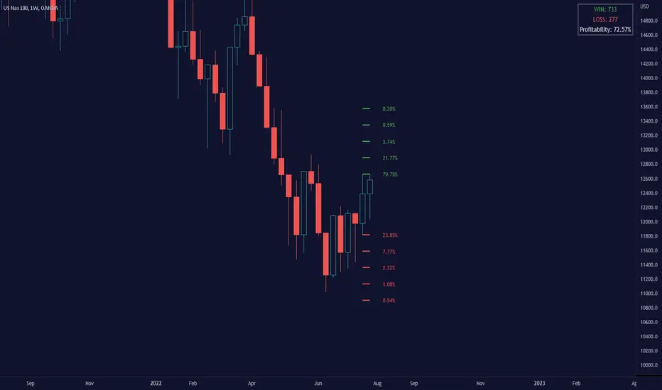
Breakout Probability (Expo)█ Overview
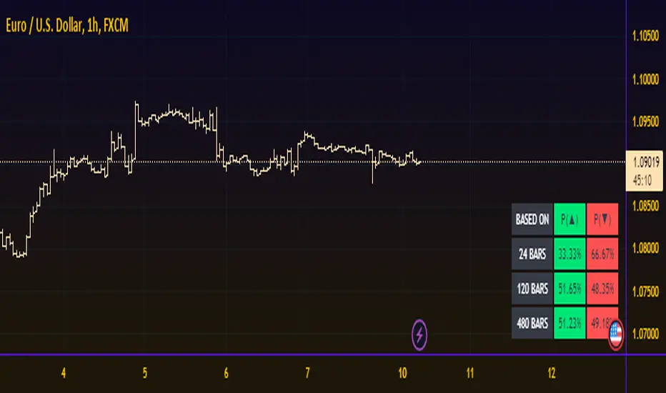
Breakout Probability is a valuable indicator that calculates the probability of a new high or low and displays it as a level with its percentage. The probability of a new high and low is backtested, and the results are shown in a table— a simple way to understand the next candle's likelihood of a new high or low. In addition, the indicator displays an additional four levels above and under the candle with the probability of hitting these levels.
The indicator helps traders to understand the likelihood of the next candle's direction, which can be used to set your trading bias.
█ Calculations
The algorithm calculates all the green and red candles separately depending on whether the previous candle was red or green and assigns scores if one or more lines were reached. The algorithm then calculates how many candles reached those levels in history and displays it as a percentage value on each line.
█ Example
In this example, the previous candlestick was green; we can see that a new high has been hit 72.82% of the time and the low only 28.29%. In this case, a new high was made.
█ Settings
Percentage Step
The space between the levels can be adjusted with a percentage step. 1% means that each level is located 1% above/under the previous one.
Disable 0.00% values
If a level got a 0% likelihood of being hit, the level is not displayed as default. Enable the option if you want to see all levels regardless of their values.
Number of Lines
Set the number of levels you want to display.
Show Statistic Panel
Enable this option if you want to display the backtest statistics for that a new high or low is made. (Only if the first levels have been reached or not)
█ Any Alert function call
An alert is sent on candle open, and you can select what should be included in the alert. You can enable the following options:
Ticker ID
Bias
Probability percentage
The first level high and low price
█ How to use
This indicator is a perfect tool for anyone that wants to understand the probability of a breakout and the likelihood that set levels are hit.
The indicator can be used for setting a stop loss based on where the price is most likely not to reach.
The indicator can help traders to set their bias based on probability. For example, look at the daily or a higher timeframe to get your trading bias, then go to a lower timeframe and look for setups in that direction.
-----------------
Disclaimer
The information contained in my Scripts/Indicators/Ideas/Algos/Systems does not constitute financial advice or a solicitation to buy or sell any securities of any type. I will not accept liability for any loss or damage, including without limitation any loss of profit, which may arise directly or indirectly from the use of or reliance on such information.
All investments involve risk, and the past performance of a security, industry, sector, market, financial product, trading strategy, backtest, or individual's trading does not guarantee future results or returns. Investors are fully responsible for any investment decisions they make. Such decisions should be based solely on an evaluation of their financial circumstances, investment objectives, risk tolerance, and liquidity needs.
My Scripts/Indicators/Ideas/Algos/Systems are only for educational purposes!
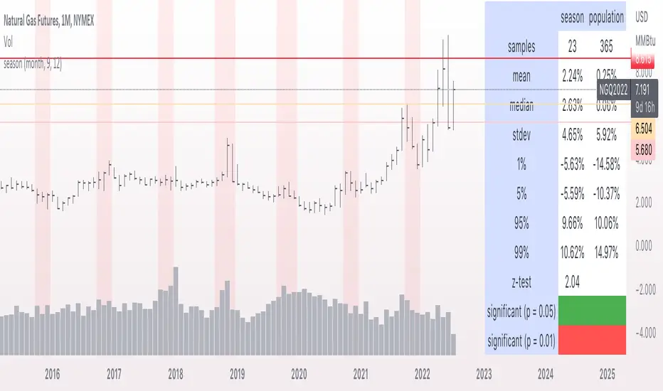
seasonThis script is meant to help verify the existence of a seasonal effect in asset returns, using a Z-test. There are three steps:
1. Think of a way to identify a season. The available methods are: by month, by week of the year, by day of the month, by day of the week, by hour of the day, and by minute of the hour.
2. Set the chart to the unit of your season. For example, if you want to check whether a crop commodity's harvest season has a seasonal implication, select "month". If you want to investigate the exchange's opening or close, select "hour".
3. Using the inputs, select the unit (e.g. "month", "dayofweek", "hour", etc.) and the range that identifies the season. The example natural gas chart has set "start" to 8 and "end" to 12 for September through December.
The test logic is as follows:
The "season" you select has a fixed length; for example, months eight through twelve has a length of four. This length is used to compute a sample mean, which is the mean return of all September-December periods in the chart. It is also used to calculate the mean/stdev of every other four-month period in the chart history. The latter is considered the "population." Using a Z-test, the script scores the difference between the sample returns and the population returns, and displays the results at two levels of significance (P = 0.05 and P = 0.01). The null hypothesis is "there is no difference between the seasonal periods and the population of ordinary periods". If the Z-score is sufficiently large or small, we can reject the null hypothesis and say that there is a seasonal effect at the given level of confidence. The output table will show green for a rejection of the null hypothesis (meaning there is a seasonal effect) or red of acceptance (there is no seasonal effect).
The seasonal periods that you have defined will be highlighted on the chart, so you can make sure they are correct. Additionally, the output table shows the mean, median, standard deviation, and top and bottom percentiles for both the seasonal and population samples.
Many news sites, twitter feeds, influences, etc. enjoy posting statistics about past returns, like "the stock market has gone up on this day 85 out of the past 100 years" and so on. Unfortunately, these posts don't tell you that many of these statistics are meaningless, as even totally random price fluctuations will cause many such interesting figures to occur. This script provides a limited means of testing some such seasonal effects so you can see if they are probably just random, or if they may have some meaning.
Note that Tradingview seems to use 1-based indexing for daily or higher timeframes, and 0-based indexing for intraday timeframes:
Months: 1-12
Weeks: 1-52
Days (of month): 1-31
Days (of week): 1-7
Hours (of day): 0-23
Minutes (of hour): 0-59
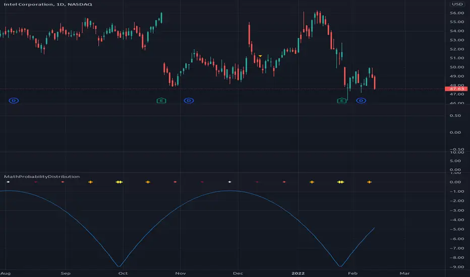
MathProbabilityDistributionLibrary "MathProbabilityDistribution"
Probability Distribution Functions.
name(idx) Indexed names helper function.
Parameters:
idx : int, position in the range (0, 6).
Returns: string, distribution name.
usage:
.name(1)
Notes:
(0) => 'StdNormal'
(1) => 'Normal'
(2) => 'Skew Normal'
(3) => 'Student T'
(4) => 'Skew Student T'
(5) => 'GED'
(6) => 'Skew GED'
zscore(position, mean, deviation) Z-score helper function for x calculation.
Parameters:
position : float, position.
mean : float, mean.
deviation : float, standard deviation.
Returns: float, z-score.
usage:
.zscore(1.5, 2.0, 1.0)
std_normal(position) Standard Normal Distribution.
Parameters:
position : float, position.
Returns: float, probability density.
usage:
.std_normal(0.6)
normal(position, mean, scale) Normal Distribution.
Parameters:
position : float, position in the distribution.
mean : float, mean of the distribution, default=0.0 for standard distribution.
scale : float, scale of the distribution, default=1.0 for standard distribution.
Returns: float, probability density.
usage:
.normal(0.6)
skew_normal(position, skew, mean, scale) Skew Normal Distribution.
Parameters:
position : float, position in the distribution.
skew : float, skewness of the distribution.
mean : float, mean of the distribution, default=0.0 for standard distribution.
scale : float, scale of the distribution, default=1.0 for standard distribution.
Returns: float, probability density.
usage:
.skew_normal(0.8, -2.0)
ged(position, shape, mean, scale) Generalized Error Distribution.
Parameters:
position : float, position.
shape : float, shape.
mean : float, mean, default=0.0 for standard distribution.
scale : float, scale, default=1.0 for standard distribution.
Returns: float, probability.
usage:
.ged(0.8, -2.0)
skew_ged(position, shape, skew, mean, scale) Skew Generalized Error Distribution.
Parameters:
position : float, position.
shape : float, shape.
skew : float, skew.
mean : float, mean, default=0.0 for standard distribution.
scale : float, scale, default=1.0 for standard distribution.
Returns: float, probability.
usage:
.skew_ged(0.8, 2.0, 1.0)
student_t(position, shape, mean, scale) Student-T Distribution.
Parameters:
position : float, position.
shape : float, shape.
mean : float, mean, default=0.0 for standard distribution.
scale : float, scale, default=1.0 for standard distribution.
Returns: float, probability.
usage:
.student_t(0.8, 2.0, 1.0)
skew_student_t(position, shape, skew, mean, scale) Skew Student-T Distribution.
Parameters:
position : float, position.
shape : float, shape.
skew : float, skew.
mean : float, mean, default=0.0 for standard distribution.
scale : float, scale, default=1.0 for standard distribution.
Returns: float, probability.
usage:
.skew_student_t(0.8, 2.0, 1.0)
select(distribution, position, mean, scale, shape, skew, log) Conditional Distribution.
Parameters:
distribution : string, distribution name.
position : float, position.
mean : float, mean, default=0.0 for standard distribution.
scale : float, scale, default=1.0 for standard distribution.
shape : float, shape.
skew : float, skew.
log : bool, if true apply log() to the result.
Returns: float, probability.
usage:
.select('StdNormal', __CYCLE4F__, log=true)
Probability ConesA probability cone is an indicator that forecasts a statistical distribution from a set point in time into the future.
Features
Forecast a Standard or Laplace distribution.
Change the how many bars the cones will lookback and sample in their calculations.
Set how many bars to forecast the cones.
Let the cones follow price from a set number of bars back.
Anchor the cones and they will not update from their last location.
Show or hide any set of cones.
Change the deviation used of any cone's upper or lower line.
Change any line's color, style, or width.
Change or toggle the fill colors between any two cone lines.
Basic Interpretations
First, there is an assumption that the distribution starting from the cone's origin, based on the number of historical bars sampled, is likely to represent the distribution of future price.
Price typically hangs around the mean.
About 68% of price stays within the first deviation cones.
About 95% of price stays within the second deviation cones.
About 99.7% of price stays within the third deviation cones.
When price is between the first and second deviation cones, there is a higher probability for a reversal.
However, strong momentum while above or below the first deviation can indicate a trend where price maintains itself past the first deviation. For this reason it's recommended to use a momentum indicator alongside the cones.
There is no mean reversion assumption when price deviates. Price can continue to stay deviated.
It's recommended that the cones are placed at the beginning of calendar periods. Like the month, week, or day.
Be mindful when using the cones on various timeframes. As the lookback setting, which selects the number of bars back to load from the cone's origin, will load the number of bars back based on the current timeframe.
Second Deviation Strategy
How to react when price goes beyond the second deviation is contingent on your trading position.
If you are holding a losing trade and price has moved past the second deviation, it could be time to stop trading and exit.
If you are holding a winning trade and price has moved past the second deviation, it would be best to look at exit strategies to capitalize on the outperformance.
If price has moved beyond the second deviation and you hold no position, then do not open any new trades.

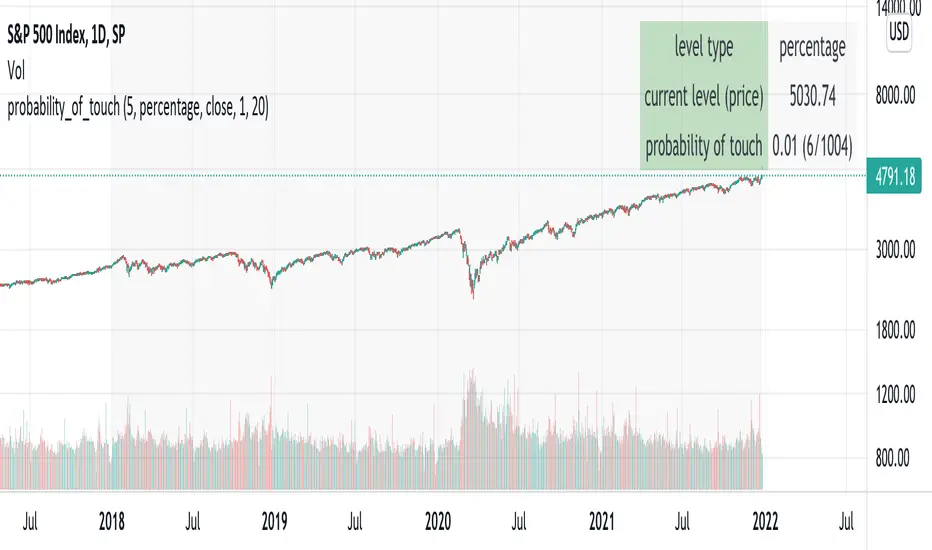
probability_of_touchBased on historical data (rather than theory), calculates the probability of a price level being "touched" within a given time frame. A "touch" means that price exceeded that level at some point. The parameters are:
- level: the "level" to be touched. it can be a number of points, percentage points, or standard deviations away from the mark price. a positive level is above the mark price, and a negative level is below the mark price.
- type: determines the meaning of the "level" parameter. "price" means price points (i.e. the numbers you see on the chart). "percentage" is expressed as a whole number, not a fraction. "stdev" means number of standard deviations, which is computed from recent realized volatlity.
- mark: the point from which the "level" is measured.
- length: the number of days within which the level must be touched.
- window: the number of days used to compute realized volatility. this parameter is only used when "type" is "stdev".
- debug: displays a fuchsia "X" over periods that touched the level. note that only a limited number of labels can be drawn.
- start: only include data after this time in the calculation.
- end: only include data before this time in the calculation.
Example: You want to know how many times Apple stock fell $1 from its closing price the next day, between 2020-02-26 and today. Use the following parameters:
level: -1
type: price
mark: close
length: 1
window:
debug:
start: 2020-02-26
end:
How does the script work? On every bar, the script looks back "length" days and sees if any day exceeded the "mark" price from "length" days ago, plus the limit. The probability is the ratio of such periods wherein price exceeded the limit to the total number of periods.
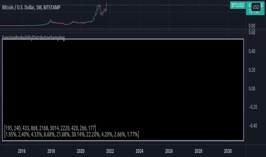
FunctionProbabilityDistributionSamplingLibrary "FunctionProbabilityDistributionSampling"
Methods for probability distribution sampling selection.
sample(probabilities) Computes a random selected index from a probability distribution.
Parameters:
probabilities : float array, probabilities of sample.
Returns: int.
FunctionSMCMCLibrary "FunctionSMCMC"
Methods to implement Markov Chain Monte Carlo Simulation (MCMC)
markov_chain(weights, actions, target_path, position, last_value) a basic implementation of the markov chain algorithm
Parameters:
weights : float array, weights of the Markov Chain.
actions : float array, actions of the Markov Chain.
target_path : float array, target path array.
position : int, index of the path.
last_value : float, base value to increment.
Returns: void, updates target array
mcmc(weights, actions, start_value, n_iterations) uses a monte carlo algorithm to simulate a markov chain at each step.
Parameters:
weights : float array, weights of the Markov Chain.
actions : float array, actions of the Markov Chain.
start_value : float, base value to start simulation.
n_iterations : integer, number of iterations to run.
Returns: float array with path.

ProbabilityLibrary "Probability"
erf(value) Complementary error function
Parameters:
value : float, value to test.
Returns: float
ierf_mcgiles(value) Computes the inverse error function using the Mc Giles method, sacrifices accuracy for speed.
Parameters:
value : float, -1.0 >= _value >= 1.0 range, value to test.
Returns: float
ierf_double(value) computes the inverse error function using the Newton method with double refinement.
Parameters:
value : float, -1. > _value > 1. range, _value to test.
Returns: float
ierf(value) computes the inverse error function using the Newton method.
Parameters:
value : float, -1. > _value > 1. range, _value to test.
Returns: float
complement(probability) probability that the event will not occur.
Parameters:
probability : float, 0 >=_p >= 1, probability of event.
Returns: float
entropy_gini_impurity_single(probability) Gini Inbalance or Gini index for a given probability.
Parameters:
probability : float, 0>=x>=1, probability of event.
Returns: float
entropy_gini_impurity(events) Gini Inbalance or Gini index for a series of events.
Parameters:
events : float , 0>=x>=1, array with event probability's.
Returns: float
entropy_shannon_single(probability) Entropy information value of the probability of a single event.
Parameters:
probability : float, 0>=x>=1, probability value.
Returns: float, value as bits of information.
entropy_shannon(events) Entropy information value of a distribution of events.
Parameters:
events : float , 0>=x>=1, array with probability's.
Returns: float
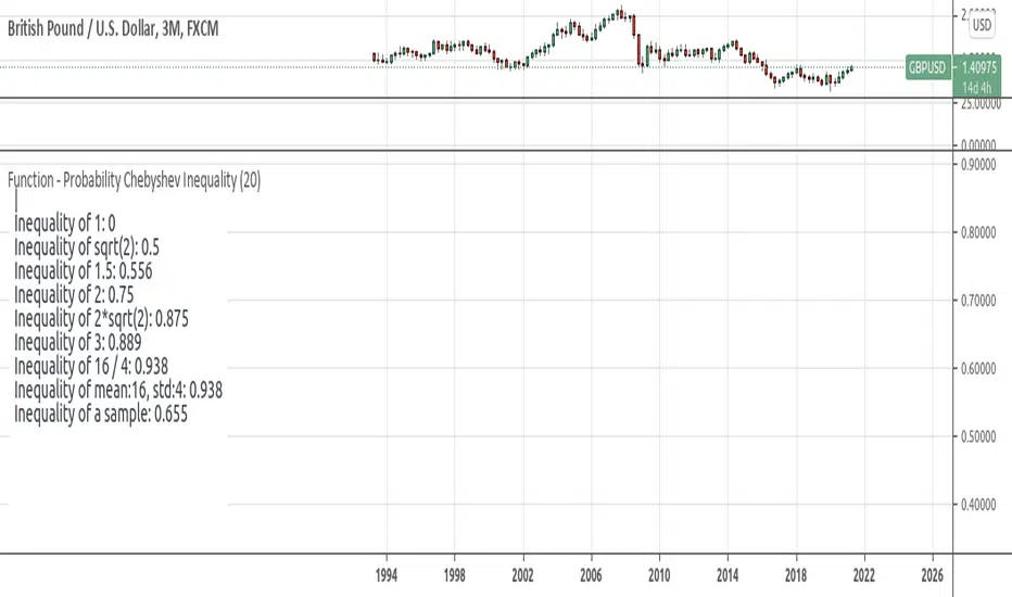
inequality_chebyshev(n_stdeviations) Calculates Chebyshev Inequality.
Parameters:
n_stdeviations : float, positive over or equal to 1.0
Returns: float
inequality_chebyshev_distribution(mean, std) Calculates Chebyshev Inequality.
Parameters:
mean : float, mean of a distribution
std : float, standard deviation of a distribution
Returns: float
inequality_chebyshev_sample(data_sample) Calculates Chebyshev Inequality for a array of values.
Parameters:
data_sample : float , array of numbers.
Returns: float
intersection_of_independent_events(events) Probability that all arguments will happen when neither outcome
is affected by the other (accepts 1 or more arguments)
Parameters:
events : float , 0 >= _p >= 1, list of event probabilities.
Returns: float
union_of_independent_events(events) Probability that either one of the arguments will happen when neither outcome
is affected by the other (accepts 1 or more arguments)
Parameters:
events : float , 0 >= _p >= 1, list of event probabilities.
Returns: float
mass_function(sample, n_bins) Probabilities for each bin in the range of sample.
Parameters:
sample : float , samples to pool probabilities.
n_bins : int, number of bins to split the range
@return float
cumulative_distribution_function(mean, stdev, value) Use the CDF to determine the probability that a random observation
that is taken from the population will be less than or equal to a certain value.
Or returns the area of probability for a known value in a normal distribution.
Parameters:
mean : float, samples to pool probabilities.
stdev : float, number of bins to split the range
value : float, limit at which to stop.
Returns: float
transition_matrix(distribution) Transition matrix for the suplied distribution.
Parameters:
distribution : float , array with probability distribution. ex:.
Returns: float
diffusion_matrix(transition_matrix, dimension, target_step) Probability of reaching target_state at target_step after starting from start_state
Parameters:
transition_matrix : float , "pseudo2d" probability transition matrix.
dimension : int, size of the matrix dimension.
target_step : number of steps to find probability.
Returns: float
state_at_time(transition_matrix, dimension, start_state, target_state, target_step) Probability of reaching target_state at target_step after starting from start_state
Parameters:
transition_matrix : float , "pseudo2d" probability transition matrix.
dimension : int, size of the matrix dimension.
start_state : state at which to start.
target_state : state to find probability.
target_step : number of steps to find probability.

Probability Distribution HistogramProbability Distribution Histogram
During data exploration it is often useful to plot the distribution of the data one is exploring. This indicator plots the distribution of data between different bins.
Essentially, what we do is we look at the min and max of the entire data set to determine its range. When we have the range of the data, we decide how many bins we want to divide this range into, so that the more bins we get, the smaller the range (a.k.a. width) for each bin becomes. We then place each data point in its corresponding bin, to see how many of the data points end up in each bin. For instance, if we have a data set where the smallest number is 5 and the biggest number is 105, we get a range of 100. If we then decide on 20 bins, each bin will have a width of 5. So the left-most bin would therefore correspond to values between 5 and 10, and the bin to the right would correspond to values between 10 and 15, and so on.
Once we have distributed all the data points into their corresponding bins, we compare the count in each bin to the total number of data points, to get a percentage of the total for each bin. So if we have 100 data points, and the left-most bin has 2 data points in it, that would equal 2%. This is also known as probability mass (or well, an approximation of it at least, since we're dealing with a bin, and not an exact number).
Usage
This is not an indicator that will give you any trading signals. This indicator is made to help you examine data. It can take any input you give it and plot how that data is distributed.
The indicator can transform the data in a few ways to help you get the most out of your data exploration. For instance, it is usually more accurate to use logarithmic data than raw data, so there is an option to transform the data using the natural logarithmic function. There is also an option to transform the data into %-Change form or by using data differencing.
Another option that the indicator has is the ability to trim data from the data set before plotting the distribution. This can help if you know there are outliers that are made up of corrupted data or data that is not relevant to your research.
I also included the option to plot the normal distribution as well, for comparison. This can be useful when the data is made up of residuals from a prediction model, to see if the residuals seem to be normally distributed or not.

Probability TableThe script is inspired by user NickbarComb, I suggested checking out his Price Convergence script.
Basically, this script plots a table containing the probability of the current candle closing either higher or lower based on user-define past period.
Hope that it will be helpful.
Function - Probability Chebyshev Inequalityfunction to calculate Chebyshev Inequality. wich can be used to compute the probability that we will diverge from what we expect to obtain.
reference:
- www.omnicalculator.com
- github.com
- statisticstopics.wordpress.com
- en.wikipedia.org
Function - Entropy Gini Indexfunction to retrieve Gini Impurity / Gini Index.
reference:
- victorzhou.com
- en.wikipedia.org

Function - Shannon Entropyfunctions for shannon's entropy
reference:
- en.wiktionary.org
- machinelearningmastery.com

test - event distributiondisplays the distribution of the outcome of a event over the last event.
similar to this script:


test - delta distributiona test case for the KDE function on price delta.
the KDE function can be used to quickly check or confirm edge cases of the trading systems conditionals.

The Bayesian Q OscillatorFirst of all the biggest thanks to @tista and @KivancOzbilgic for publishing their open source public indicators Bayesian BBSMA + nQQE Oscillator. And a mighty round of applause for @MarkBench for once again being my superhero pinescript guy that puts these awesome combination Ideas and ES stradegies in my head together. Now let me go ahead and explain what we have here.
I am gonna call it the Bayesian Q Oscillator I suppose. The goal of the script is to solve an issue both indicators on their own suffer from. QQE signals are not new and often the problem has always been false signals for them. They are good for scalping but the difference between a quality move and a small to nearly nonexistent move following a signal is not so clear. Kivanc made his normalized version to help reduce this problem by adding colors to his histogram type verision that would essentially represent if price was a trending move or in a ranging structure. As you can see I have kept this Idea but instead opted for lines as the oscillator. two yellow line (default color) is a ranging sideways area and when there is red or green it is trending up or down. I wanted to take this to the next level with combining the Bayesian probability oscillator that tista put together.
The Bayesian indicator is the opposite for its issue as it is a probability indicator that shows which candle or price movement is more likely to come next. Red rising means possibly down move soon and green means up soon. I will not go into the complex details of this indicator but will suggest others take a look at his and others to understand the idea behind them. The point I am driving at is that it show probabilities or likelyhood without the most effecient signal device to match it. This original was line form and now it is background filled colors.
The idea. is that you can potentially get some stronger and more accurate reversal signals with these two paired together. when you see a sell signal or cross with the towering or rising red... maybe it is a good jump potentially. The same for green. At the same time it is a double added filter effect from just having yellow represent it is ranging... but now if you get a buy signal (example) and have yellow lines (example) along wi5h a red rising or mountain color background... it not only is an indication of ranging, but also that there is potentially even a counter move coming based on the probabilities. Also if you get into a good trade and see dual yellow qqe crosses with no color represented by the bayesian background... it is possible it might only be noise.
I have found them to work decently in the 1 hour timframe. Let me know your experience.
I hope everyone takes a look at the originals to understand them. Full credit goes to those guys for this to be here. Let me know how it is working out for you.
Here are the original links.
bayesian
Normalized QQE

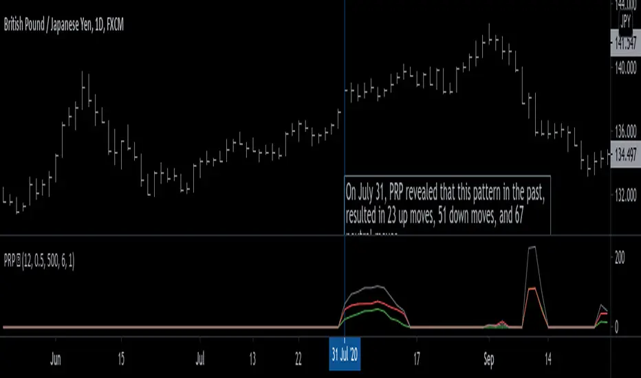
Pattern Recognition Probabilities [racer8]Brief 🌟
Pattern Recognition Probabilities (PRP) is a REALLY smart indicator. It uses the correlation coefficient formula to determine if the current set of bars resembles that of past patterns. It counts the number of times the current pattern has occurred in the past and looks at how it performed historically to determine the probability of an up move, down move, or neutral move.
I'd like to say, I'm proud of this indicator 😆🤙 This is the SMARTEST indicator I have ever made 🧠🧠🧠
Note: PRP doesn't give you actual probabilities, but gives you instead the historical occurrences of up, down, and neutral moves that resulted after the pattern. So you can calculate probabilities based on these valuable statistics. So for example, PRP can tell you this pattern has historically resulted in 55 up moves, 20 down moves, and 60 neutral moves.
Parameters 🌟
You can adjust the Pattern length, Minimum correlation, Statistics lookback, Exit after time, and Atr multiplier parameters.
Pattern length - determines how long the pattern is
Minimum correlation - determines the minimum correlation coefficient needed to pass as a similiar enough pattern.
Statistics lookback - lookback period for gathering all the patterns in the past.
Exit after time - determines when exit occurred (number of periods after pattern) ; is the point that represents the pattern's result.
Atr multiplier - determines minimum atr move needed to qualify whether result was an up/down move or a neutral move. If a particular historical pattern resulted in a move that was less than the min atr, then it is recorded as a neutral move in the statistics.
Thanks for reading! 🙏
Good luck 🍀 Stay safe 😷 Drink lots of water💧
Enjoy! 🥳 and Hit the like button! 👍
Expected Range and SkewThis is an open source and updated version of my previous "Confidence Interval" script. This script provides you with the expected range over a given time period in the future and the skew of that range. For example, if you wanted to know the expected 1 standard deviation range of MSFT over the next 20 days, this will tell you that. Additionally, this script will also tell you the skew of the expected range.
How to use this script:
1) Enter the length, this will determine the number of data points used in the calculation of the expected range.
2) Enter the amount of time you want projected forward in minutes, hours, and days.
3) Input standard deviation of the expected range.
4) Pick the type of data you want shown from the dropdown menu. Your choices are either the expected range or the skew of the expected range.
5) Enter the x and y coordinates of the label (optional). This is useful so it doesn't impede your view of the plot.
Here are a few notes about this script:
First, the expected range line gives you the width of said range (upper bound - lower bound), and the label will tell you specifically what the upper and lower bounds of the expected range are.
Second, this script will work on any of the default timeframes, but you need to be careful with how far out you try to project the expected range depending on the timeframe you're using. For example, if you're using the 1min timeframe, it probably won't do you any good trying to project the expected range over the next 20 days; or if you're using the daily timeframe it doesn't make sense to try to project the expected range for the next 5 hours. You can tell if the time horizon you're trying to project doesn't work well with the chart timeframe you're using if the current price is outside of either the upper or lower bounds provided in the label. If the current price is within the upper and lower bounds provided in the label, then the time horizon that you're projecting over is reasonable for the chart timeframe you're using.
Third, this script does not countdown automatically, so the time provided in the label will stay the same. For example, in the picture above, the expected range of Dow Futures over the next 23 days from January 12th, 2021 is calculated. But when tomorrow comes it won't count down to 22 days, instead it will show the range over the next 23 days from January 13th, 2021. So if you want the time horizon to change as time goes on you will have to update this yourself manually.
Lastly, if you try to set an alert on this script, you will get a warning about it possibly repainting. This is because of the label, not the plot itself. The label constantly updates itself, which triggers the warning. I tested setting alerts on this script both with and without the inclusion of the label, and without the label the repainting warning did not occur. So remember, if you set an alert on this script you will get a warning about it possibly repainting, but this is because of the label constantly updating, not the plot itself.